Introduction
This is a tale of two approaches to regular expression matching.
One of them is in widespread use in the
standard interpreters for many languages, including Perl.
The other is used only in a few places, notably most implementations
of awk and grep.
The two approaches have wildly different
performance characteristics:
 | 
| |
Time to match a?nan against an
| ||
Let's use superscripts to denote string repetition,
so that
a?3a3
is shorthand for
a?a?a?aaa.
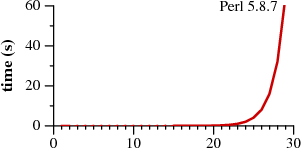
The two graphs plot the time required by each approach
to match the regular expression
a?nan
against the string an.
Notice that Perl requires over sixty seconds to match
a 29-character string.
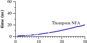
The other approach, labeled Thompson NFA for
reasons that will be explained later,
requires twenty microseconds to match the string.
That's not a typo. The Perl graph plots time in seconds,
while the Thompson NFA graph plots time in microseconds:
the Thompson NFA implementation
is a million times faster than Perl
when running on a miniscule 29-character string.
The trends shown in the graph continue: the
Thompson NFA handles a 100-character string in under 200 microseconds,
while Perl would require over 1015 years.
(Perl is only the most conspicuous example of a large
number of popular programs that use the same algorithm;
the above graph could have been Python, or PHP, or Ruby,
or many other languages. A more detailed
graph later in this article presents data for other implementations.)
It may be hard to believe the graphs: perhaps you've used Perl,
and it never seemed like regular expression matching was
particularly slow.
Most of the time, in fact, regular expression matching in Perl
is fast enough.
As the graph shows, though, it is possible
to write so-called “pathological” regular expressions that
Perl matches very very slowly.
In contrast, there are no regular expressions that are
pathological for the Thompson NFA implementation.
Seeing the two graphs side by side prompts the question,
“why doesn't Perl use the Thompson NFA approach?”
It can, it should, and that's what the rest of this article is about.
Historically, regular expressions are one of computer science's
shining examples of how using good theory leads to good programs.
They were originally developed by theorists as a
simple computational model,
but Ken Thompson introduced them to
programmers in his implementation of the text editor QED
for CTSS.
Dennis Ritchie followed suit in his own implementation
of QED, for GE-TSS.
Thompson and Ritchie would go on to create Unix,
and they brought regular expressions with them.
By the late 1970s, regular expressions were a key
feature of the Unix landscape, in tools such as
ed, sed, grep, egrep, awk, and lex.
Today, regular expressions have also become a shining
example of how ignoring good theory leads to bad programs.
The regular expression implementations used by
today's popular tools are significantly slower
than the ones used in many of those thirty-year-old Unix tools.
This article reviews the good theory:
regular expressions, finite automata,
and a regular expression search algorithm
invented by Ken Thompson in the mid-1960s.
It also puts the theory into practice, describing
a simple implementation of Thompson's algorithm.
That implementation, less than 400 lines of C,
is the one that went head to head with Perl above.
It outperforms the more complex real-world
implementations used by
Perl, Python, PCRE, and others.
The article concludes with a discussion of how
theory might yet be converted into practice
in the real-world implementations.
Regular Expressions
Regular expressions are a notation for
describing sets of character strings.
When a particular string is in the set
described by a regular expression,
we often say that the regular expression
matches
the string.
The simplest regular expression is a single literal character.
Except for the special metacharacters
*+?()|,
characters match themselves.
To match a metacharacter, escape it with
a backslash:
\+
matches a literal plus character.
Two regular expressions can be alternated or concatenated to form a new
regular expression:
if e1 matches
s
and e2 matches
t,
then e1
|e2 matches
s
or
t,
and
e1e2
matches
st.
The metacharacters
*,
+,
and
?
are repetition operators:
e1*
matches a sequence of zero or more (possibly different)
strings, each of which match e1;
e1+
matches one or more;
e1?
matches zero or one.
The operator precedence, from weakest to strongest binding, is
first alternation, then concatenation, and finally the
repetition operators.
Explicit parentheses can be used to force different meanings,
just as in arithmetic expressions.
Some examples:
ab|cd
is equivalent to
(ab)|(cd);
ab*
is equivalent to
a(b*).
The syntax described so far is a subset of the traditional Unix
egrep
regular expression syntax.
This subset suffices to describe all regular
languages: loosely speaking, a regular language is a set
of strings that can be matched in a single pass through
the text using only a fixed amount of memory.
Newer regular expression facilities (notably Perl and
those that have copied it) have added
many new operators
and escape sequences. These additions make the regular
expressions more concise, and sometimes more cryptic, but usually
not more powerful:
these fancy new regular expressions almost always have longer
equivalents using the traditional syntax.
One common regular expression extension that
does provide additional power is called
backreferences.
A backreference like
\1
or
\2
matches the string matched
by a previous parenthesized expression, and only that string:
(cat|dog)\1
matches
catcat
and
dogdog
but not
catdog
nor
dogcat.
As far as the theoretical term is concerned,
regular expressions with backreferences
are not regular expressions.
The power that backreferences add comes at great cost:
in the worst case, the best known implementations require
exponential search algorithms,
like the one Perl uses.
Perl (and the other languages)
could not now remove backreference support,
of course, but they could employ much faster algorithms
when presented with regular expressions that don't have
backreferences, like the ones considered above.
This article is about those faster algorithms.
Finite Automata
Another way to describe sets of character strings is with
finite automata.
Finite automata are also known as state machines,
and we will use “automaton” and “machine” interchangeably.
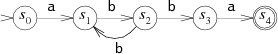
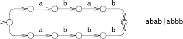
As a simple example, here is a machine recognizing
the set of strings matched by the regular expression
a(bb)+a:
A finite automaton is always in one of its states,
represented in the diagram by circles.
(The numbers inside the circles are labels to make this
discussion easier; they are not part of the machine's operation.)
As it reads the string, it switches from state to state.
This machine has two special states: the start state s0
and the matching state s4.
Start states are depicted with lone arrowheads pointing at them,
and matching states are drawn as a double circle.
The machine reads an input string one character at a time,
following arrows corresponding to the input to move from
state to state.
Suppose the input string is
abbbba.
When the machine reads the first letter of the string, the
a,
it is in the start state s0. It follows the
a
arrow to state s1.
This process repeats as the machine reads the rest of the string:
b
to
s2,
b
to
s3,
b
to
s2,
b
to
s3,
and finally
a
to
s4.
The machine ends in s4, a matching state, so it
matches the string.
If the machine ends in a non-matching state, it does not
match the string.
If, at any point during the machine's execution, there is no
arrow for it to follow corresponding to the current
input character, the machine stops executing early.
The machine we have been considering is called a
deterministic
finite automaton (DFA),
because in any state, each possible input letter
leads to at most one new state.
We can also create machines
that must choose between multiple possible next states.
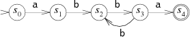
For example, this machine is equivalent to the previous
one but is not deterministic:
The machine is not deterministic because if it reads a
b
in state s2, it has multiple choices for the next state:
it can go back to s1 in hopes of seeing another
bb,
or it can go on to s3 in hopes of seeing the final
a.
Since the machine cannot peek ahead to see the rest of
the string, it has no way to know which is the correct decision.
In this situation, it turns out to be interesting to
let the machine
always guess correctly.
Such machines are called non-deterministic finite automata
(NFAs or NDFAs).
An NFA matches an input string if there is some way
it can read the string and follow arrows to a matching state.
Sometimes it is convenient to let NFAs have arrows with no
corresponding input character. We will leave these arrows unlabeled.
An NFA can, at any time, choose to follow an unlabeled arrow
without reading any input.
This NFA is equivalent to the previous two, but the unlabeled arrow
makes the correspondence with
a(bb)+a
clearest:
Converting Regular Expressions to NFAs
Regular expressions and NFAs turn out to be exactly
equivalent in power: every regular expression has an
equivalent NFA (they match the same strings) and vice versa.
(It turns out that DFAs are also equivalent in power
to NFAs and regular expressions; we will see this later.)
There are multiple ways to translate regular expressions into NFAs.
The method described here was first described by Thompson
in his 1968 CACM paper.
The NFA for a regular expression is built up from partial NFAs
for each subexpression, with a different construction for
each operator. The partial NFAs have
no matching states: instead they have one or more dangling arrows,
pointing to nothing. The construction process will finish by
connecting these arrows to a matching state.
The NFAs for matching single characters look like:
The NFA for the concatenation e1e2
connects the final arrow of the e1
machine to the start of the e2 machine:
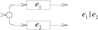
The NFA for the alternation e1
|e2
adds a new start state with a choice of either the
e1 machine or the e2 machine.
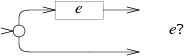
The NFA for e
? alternates the e machine with an empty path:
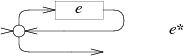
The NFA for e
* uses the same alternation but loops a
matching e machine back to the start:
The NFA for e
+ also creates a loop, but one that
requires passing through e at least once:
Counting the new states in the diagrams above, we can see
that this technique creates exactly one state per character
or metacharacter in the regular expression,
excluding parentheses.
Therefore the number of states in the final NFA is at most
equal to the length of the original regular expression.
Just as with the example NFA discussed earlier, it is always possible
to remove the unlabeled arrows, and it is also always possible to generate
the NFA without the unlabeled arrows in the first place.
Having the unlabeled arrows makes the NFA easier for us to read
and understand, and they also make the C representation
simpler, so we will keep them.
Regular Expression Search Algorithms
Now we have a way to test whether a regular expression
matches a string: convert the regular expression to an NFA
and then run the NFA using the string as input.
Remember that NFAs are endowed with the ability to guess
perfectly when faced with a choice of next state:
to run the NFA using an ordinary computer, we must find
a way to simulate this guessing.
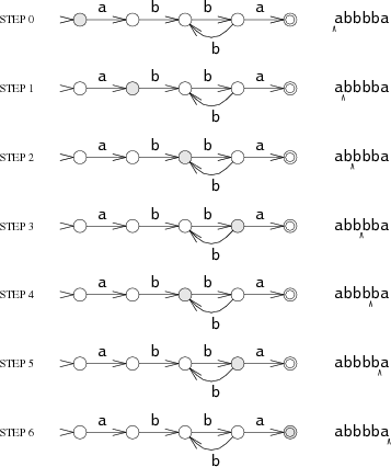
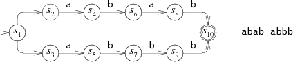
One way to simulate perfect guessing is to guess
one option, and if that doesn't work, try the other.
For example, consider the NFA for
abab|abbb
run on the string
abbb:
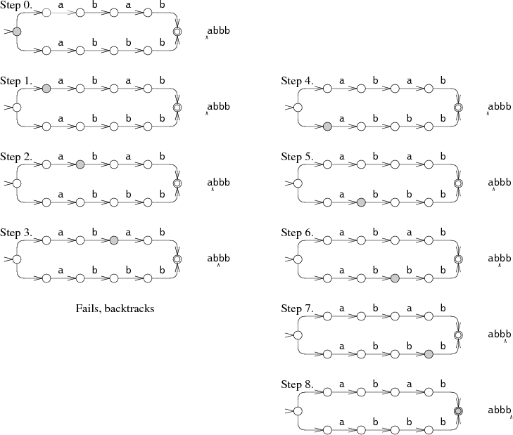
At step 0, the NFA must make a choice: try to match
abab
or
try to match
abbb?
In the diagram, the NFA tries
abab,
but that fails after step 3.
The NFA then tries the other choice, leading to step 4 and eventually a match.
This backtracking approach
has a simple recursive implementation
but can read the input string many times
before succeeding.
If the string does not match,
the machine must try
all
possible execution paths before
giving up.
The NFA tried only two different paths in the example,
but in the worst case, there can be exponentially
many possible execution paths, leading to very slow run times.
A more efficient but more complicated way to simulate perfect
guessing is to guess both options simultaneously.
In this approach, the simulation allows the machine
to be in multiple states at once. To process each letter,
it advances all the states along all the arrows that
match the letter.
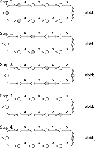
The machine starts in the start state and all the states
reachable from the start state by unlabeled arrows.
In steps 1 and 2, the NFA is in two states simultaneously.
Only at step 3 does the state set narrow down to a single state.
This multi-state approach tries both paths at the same time,
reading the input only once.
In the worst case, the NFA might be in
every
state at each step, but this results in at worst a constant amount
of work independent of the length of the string,
so arbitrarily
large input strings can be processed in linear time.
This is a dramatic improvement over the exponential time
required by the backtracking approach.
The efficiency comes from tracking the set of reachable
states but
not
which paths were used to reach them.
In an NFA with
n
nodes, there can only be
n
reachable states at any step, but there might be
2n paths through the NFA.
Implementation
Thompson introduced the multiple-state simulation approach
in his 1968 paper.
In his formulation, the states of the NFA were represented
by small machine-code sequences, and the list of possible states
was just a sequence of function call instructions.
In essence, Thompson compiled the regular expression into clever
machine code.
Forty years later, computers are much faster and the
machine code approach is not as necessary.
The following sections
present an implementation written in portable ANSI C.
The full source code (under 400 lines)
and the benchmarking scripts are
available online.
(Readers who are unfamiliar or uncomfortable with C or pointers should
feel free to read the descriptions and skip over the actual code.)
Implementation: Compiling to NFA
The first step is to compile the regular expression
into an equivalent NFA.
In our C program, we will represent an NFA as a
linked collection of
State
structures:
struct State
{
 int c;
 State *out;
 State *out1;
 int lastlist;
};
Each
State
represents one of the following three NFA fragments,
depending on the value of
c.
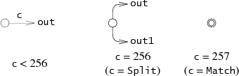
(
Lastlist
is used during execution and is explained in the next section.)
Following Thompson's paper,
the compiler builds an NFA from a regular expression in
postfix
notation with dot
(
.) added
as an explicit concatenation operator.
A separate function
re2post
rewrites infix regular expressions like
“a(bb)+a”
into equivalent postfix expressions like
“abb.+.a.”.
(A “real” implementation would certainly
need to use dot as the “any character” metacharacter
rather than as a concatenation operator.
A real implementation would also probably build the
NFA during parsing rather than build an explicit postfix expression.
However, the postfix version is convenient and follows
Thompson's paper more closely.)
As the compiler scans the postfix expression, it maintains
a stack of computed NFA fragments.
Literals push new NFA fragments onto the stack, while
operators pop fragments off the stack and then
push a new fragment.
For example,
after compiling the
abb in abb.+.a.,
the stack contains NFA fragments for
a,
b,
and
b.
The compilation of the
.
that follows pops the two
b
NFA fragment from the stack and pushes an NFA fragment for the
concatenation
bb..
Each NFA fragment is defined by its start state and its
outgoing arrows:
struct Frag
{
 State *start;
 Ptrlist *out;
};
Start
points at the start state for the fragment,
and
out
is a list of pointers to
State*
pointers that are not yet connected to anything.
These are the dangling arrows in the NFA fragment.
Some helper functions manipulate pointer lists:
Ptrlist *list1(State **outp);
Ptrlist *append(Ptrlist *l1, Ptrlist *l2);

void patch(Ptrlist *l, State *s);
List1
creates a new pointer list containing the single pointer
outp.
Append
concatenates two pointer lists, returning the result.
Patch
connects the dangling arrows in the pointer list
l
to the state
s:
it sets
*outp
=
s
for each pointer
outp
in
l.
Given these primitives and a fragment stack,
the compiler is a simple loop over the postfix expression.
At the end, there is a single fragment left:
patching in a matching state completes the NFA.
State*
post2nfa(char *postfix)
{
 char *p;
 Frag stack[1000], *stackp, e1, e2, e;
 State *s;

 #define push(s) *stackp++ = s
 #define pop()   *--stackp

 stackp = stack;
 for(p=postfix; *p; p++){
  switch(*p){
  /* compilation cases, described below */
  }
 }

 e = pop();
 patch(e.out, matchstate);
 return e.start;
}
The specific compilation cases mimic the translation
steps described earlier.
Literal characters:
default: s = state(*p, NULL, NULL); push(frag(s, list1(&s->out)); break; | |
Catenation:
case '.': e2 = pop(); e1 = pop(); patch(e1.out, e2.start); push(frag(e1.start, e2.out)); break; | |
Alternation:
case '|': e2 = pop(); e1 = pop(); s = state(Split, e1.start, e2.start); push(frag(s, append(e1.out, e2.out))); break; | 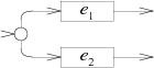
|
Zero or one:
case '?': e = pop(); s = state(Split, e.start, NULL); push(frag(s, append(e.out, list1(&s->out1)))); break; | 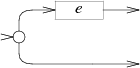
|
Zero or more:
case '*': e = pop(); s = state(Split, e.start, NULL); patch(e.out, s); push(frag(s, list1(&s->out1))); break; | 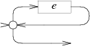
|
One or more:
case '+': e = pop(); s = state(Split, e.start, NULL); patch(e.out, s); push(frag(e.start, list1(&s->out1))); break; | 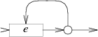
|
Implementation: Simulating the NFA
Now that the NFA has been built, we need to simulate it.
The simulation requires tracking
State
sets, which are stored as a simple array list:
struct List
{
 State **s;
 int n;
};
The simulation uses two lists:
clist
is the current set of states that the NFA is in,
and
nlist
is the next set of states that the NFA will be in,
after processing the current character.
The execution loop initializes
clist
to contain just the start state and then
runs the machine one step at a time.
int
match(State *start, char *s)
{
 List *clist, *nlist, *t;

 /* l1 and l2 are preallocated globals */
 clist = startlist(start, &l1);
 nlist = &l2;
 for(; *s; s++){
  step(clist, *s, nlist);
  t = clist; clist = nlist; nlist = t; /* swap clist, nlist */
 }
 return ismatch(clist);
}
To avoid allocating on every iteration of the loop,
match
uses two preallocated lists
l1
and
l2
as
clist
and
nlist,
swapping the two after each step.
If the final state list contains the matching state,
then the string matches.
int
ismatch(List *l)
{
 int i;

 for(i=0; i<l->n; i++)
  if(l->s[i] == matchstate)
   return 1;
 return 0;
}
Addstate
adds a state to the list,
but not if it is already on the list.
Scanning the entire list for each add would be inefficient;
instead the variable
listid
acts as a list generation number.
When
addstate
adds
s
to a list,
it records
listid
in
s->lastlist.
If the two are already equal,
then
s
is already on the list being built.
Addstate
also follows unlabeled arrows:
if
s
is a
Split
state with two unlabeled arrows to new states,
addstate
adds those states to the list instead of
s.
void
addstate(List *l, State *s)
{
 if(s == NULL || s->lastlist == listid)
  return;
 s->lastlist = listid;
 if(s->c == Split){
  /* follow unlabeled arrows */
  addstate(l, s->out);
  addstate(l, s->out1);
  return;
 }
 l->s[l->n++] = s;
}
Startlist
creates an initial state list by adding just the start state:
List*
startlist(State *s, List *l)
{
 listid++;
 l->n = 0;
 addstate(l, s);
 return l;
}
Finally,
step
advances the NFA past a single character, using
the current list
clist
to compute the next list
nlist.
void
step(List *clist, int c, List *nlist)
{
 int i;
 State *s;

 listid++;
 nlist->n = 0;
 for(i=0; i<clist->n; i++){
  s = clist->s[i];
  if(s->c == c)
   addstate(nlist, s->out);
 }
}
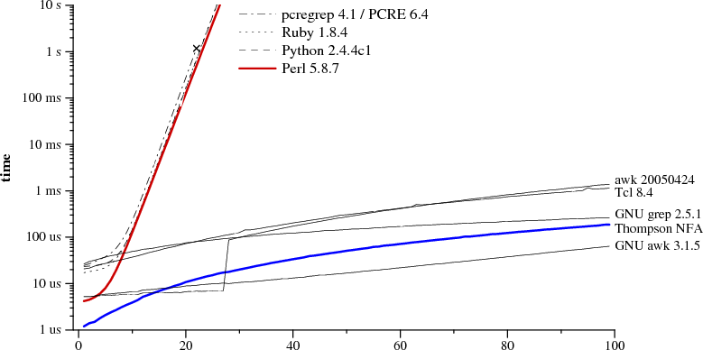
Performance
The C implementation just described was not written with performance in mind.
Even so, a slow implementation of a linear-time algorithm
can easily outperform a fast implementation of an
exponential-time algorithm once the exponent is large enough.
Testing a variety of popular regular expression engines on
a so-called pathological regular expression demonstrates this nicely.
Consider the regular expression
a?nan.
It matches the string
an
when the
a?
are chosen not to match any letters,
leaving the entire string to be matched by the
an.
Backtracking regular expression implementations
implement the zero-or-one
?
by first trying one and then zero.
There are
n
such choices to make, a total of
2n possibilities.
Only the very last
possibility—choosing zero for all the ?—will lead to a match.
The backtracking approach thus requires
O(2n) time, so it will not scale much beyond n=25.
In contrast, Thompson's algorithm maintains state lists of length
approximately n and processes the string, also of length n,
for a total of O(n2) time.
(The run time is superlinear,
because we are not keeping the regular expression constant
as the input grows.
For a regular expression of length m run on text of length n,
the Thompson NFA requires O(mn) time.)
The following graph plots time required to check whether
a?nan
matches
an:
regular expression and text size n a?nan
matching
an
|
Notice that the graph's y-axis has a logarithmic scale,
in order to be able to see a wide variety of times on a single graph.
From the graph it is clear that Perl, PCRE, Python, and Ruby are
all using recursive backtracking.
PCRE stops getting the right answer at
n=23,
because it aborts the recursive backtracking after a maximum number
of steps.
As of Perl 5.6, Perl's regular expression engine is
said to memoize
the recursive backtracking search, which should, at some memory cost,
keep the search from taking exponential amounts of time
unless backreferences are being used.
As the performance graph shows, the memoization is not complete:
Perl's run time grows exponentially even though there
are no backreferences
in the expression.
Although not benchmarked here, Java uses a backtracking
implementation too.
In fact, the
java.util.regex
interface requires a backtracking
implementation, because arbitrary Java code
can be substituted into the matching path.
PHP uses the PCRE library.
The thick blue line is the C implementation of Thompson's algorithm given above.
Awk, Tcl, GNU grep, and GNU awk
build DFAs, either precomputing them or using the on-the-fly
construction described in the next section.
Some might argue that this test is unfair to
the backtracking implementations, since it focuses on an
uncommon corner case.
This argument misses the point:
given a choice between an implementation
with a predictable, consistent, fast running time on all inputs
or one that usually runs quickly but can take
years of CPU time (or more) on some inputs,
the decision should be easy.
Also, while examples as dramatic as this one
rarely occur in practice, less dramatic ones do occur.
Examples include using
(.*)
(.*)
(.*)
(.*)
(.*)
to split five space-separated fields, or using
alternations where the common cases
are not listed first.
As a result, programmers often learn which constructs are
expensive and avoid them, or they turn to so-called
optimizers.
Using Thompson's NFA simulation does not require such adaptation:
there are no expensive regular expressions.
Caching the NFA to build a DFA
Recall that DFAs are more efficient to execute than NFAs,
because DFAs are only ever in one state at a time: they never
have a choice of multiple next states.
Any NFA can be converted into an equivalent DFA
in which each DFA state corresponds to a
list of NFA states.
For example, here is the NFA we used earlier for
abab|abbb,
with state numbers added:
The equivalent DFA would be:
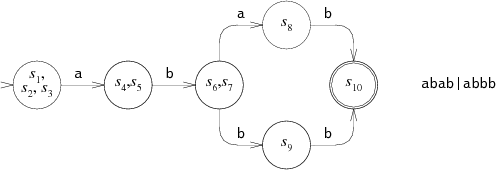
Each state in the DFA corresponds to a list of
states from the NFA.
In a sense, Thompson's NFA simulation is
executing the equivalent DFA: each
List
corresponds to some DFA state,
and the
step
function is computing, given a list and a next character,
the next DFA state to enter.
Thompson's algorithm simulates the DFA by
reconstructing each DFA state as it is needed.
Rather than throw away this work after each step,
we could cache the
Lists
in spare memory, avoiding the cost of repeating the computation
in the future
and essentially computing the equivalent DFA as it is needed.
This section presents the implementation of such an approach.
Starting with the NFA implementation from the previous section,
we need to add less than 100 lines to build a DFA implementation.
To implement the cache, we first introduce a new data type
that represents a DFA state:
struct DState
{
 List l;
 DState *next[256];
 DState *left;
 DState *right;
};
A
DState
is the cached copy of the list
l.
The array
next
contains pointers to the next state for each
possible input character:
if the current state is
d
and the next input character is
c,
then
d->next[c]
is the next state.
If
d->next[c]
is null, then the next state has not been computed yet.
Nextstate
computes, records, and returns the next state
for a given state and character.
The regular expression match follows
d->next[c]
repeatedly, calling
nextstate
to compute new states as needed.
int
match(DState *start, char *s)
{
 int c;
 DState *d, *next;

 d = start;
 for(; *s; s++){
  c = *s & 0xFF;
  if((next = d->next[c]) == NULL)
   next = nextstate(d, c);
  d = next;
 }
 return ismatch(&d->l);
}
All the
DStates
that have been computed need to be saved in a
structure that lets us look up a
DState
by its
List.
To do this, we arrange them
in a binary tree
using the sorted
List
as the key.
The
dstate
function returns the
DState
for a given
List,
allocating one if necessary:
DState*
dstate(List *l)
{
 int i;
 DState **dp, *d;
 static DState *alldstates;

 qsort(l->s, l->n, sizeof l->s[0], ptrcmp);

 /* look in tree for existing DState */
 dp = &alldstates;
 while((d = *dp) != NULL){
  i = listcmp(l, &d->l);
  if(i < 0)
   dp = &d->left;
  else if(i > 0)
   dp = &d->right;
  else
   return d;
 }

 /* allocate, initialize new DState */
 d = malloc(sizeof *d + l->n*sizeof l->s[0]);
 memset(d, 0, sizeof *d);
 d->l.s = (State**)(d+1);
 memmove(d->l.s, l->s, l->n*sizeof l->s[0]);
 d->l.n = l->n;

 /* insert in tree */
 *dp = d;
 return d;
}
Nextstate runs the NFA
step
and returns the corresponding
DState:
DState*
nextstate(DState *d, int c)
{
 step(&d->l, c, &l1);
 return d->next[c] = dstate(&l1);
}
Finally, the DFA's start state is the
DState
corresponding to the NFA's start list:
DState*
startdstate(State *start)
{
 return dstate(startlist(start, &l1));
}
(As in the NFA simulation,
l1
is a preallocated
List.)
The
DStates
correspond to DFA states, but the DFA is only built as needed:
if a DFA state has not been encountered during the search,
it does not yet exist in the cache.
An alternative would be to compute the entire DFA at once.
Doing so would make
match
a little faster by removing the conditional branch,
but at the cost of increased startup time and
memory use.
One might also worry about bounding the amount of
memory used by the on-the-fly DFA construction.
Since the
DStates
are only a cache of the
step
function, the implementation of
dstate
could choose to throw away the entire DFA so far
if the cache grew too large.
This cache replacement policy
only requires a few extra lines of code in
dstate
and in
nextstate,
plus around 50 lines of code for memory management.
An implementation is
available online.
(Awk
uses a similar limited-size cache strategy,
with a fixed limit of 32 cached states; this explains the discontinuity
in its performance at n=28 in the graph above.)
NFAs derived from regular expressions
tend to exhibit good locality: they visit the same states
and follow the same transition arrows over and over
when run on most texts.
This makes the caching worthwhile: the first time an arrow
is followed, the next state must be computed as in the NFA
simulation, but future traversals of the arrow are just
a single memory access.
Real DFA-based implementations can make use
of additional optimizations to run even faster.
A companion article (not yet written) will explore
DFA-based regular expression implementations in more detail.
Real world regular expressions
Regular expression usage in real programs
is somewhat more complicated than what the regular expression
implementations described above can handle.
This section briefly describes the common complications;
full treatment of any of these is beyond the scope of this
introductory article.
Character classes.
A character class, whether
[0-9]
or
\w
or
. (dot),
is just a concise representation of an alternation.
Character classes can be expanded into alternations
during compilation, though it is more efficient to add
a new kind of NFA node to represent them explicitly.
POSIX
defines special character classes
like [[:upper:]] that change meaning
depending on the current locale, but the hard part of
accommodating these is determining their meaning,
not encoding that meaning into an NFA.
Escape sequences.
Real regular expression syntaxes need to handle
escape sequences, both as a way to match metacharacters
(
\(,
\),
\\,
etc.)
and to specify otherwise difficult-to-type characters such as
\n.
Counted repetition.
Many regular expression implementations provide a counted
repetition operator
{n}
to match exactly
n
strings matching a pattern;
{n,m}
to match at least
n
but no more than
m;
and
{n,}
to match
n
or more.
A recursive backtracking implementation can implement
counted repetition using a loop; an NFA or DFA-based
implementation must expand the repetition:
e{3}
expands to
eee;
e{3,5}
expands to
eeee?e?,
and
e{3,}
expands to
eee+.
Submatch extraction.
When regular expressions are used for splitting or parsing strings,
it is useful to be able to find out which sections of the input string
were matched by each subexpression.
After a regular expression like
([0-9]+-[0-9]+-[0-9]+)
([0-9]+:[0-9]+)
matches a string (say a date and time),
many regular expression engines make the
text matched by each parenthesized expression
available.
For example, one might write in Perl:
if(/([0-9]+-[0-9]+-[0-9]+) ([0-9]+:[0-9]+)/){
 print "date: $1, time: $2\n";
}
The extraction of submatch boundaries has been mostly ignored
by computer science theorists, and it is perhaps the most
compelling argument for using recursive backtracking.
However, Thompson-style algorithms can be adapted to
track submatch boundaries without giving up efficient performance.
The Eighth Edition Unix
regexp(3)
library implemented such an algorithm as early as 1985,
though as explained below,
it was not very widely used or even noticed.
Unanchored matches.
This article has assumed that regular expressions
are matched against an entire input string.
In practice, one often wishes to find a substring
of the input that matches the regular expression.
Unix tools traditionally return the longest matching substring
that starts at the leftmost possible point in the input.
An unanchored search for
e
is a special case
of submatch extraction: it is like searching for
.*(e).*
where the first
.*
is constrained to match as short a string as possible.
Non-greedy operators.
In traditional Unix regular expressions, the repetition operators
?,
*,
and
+
are defined to match as much of the string as possible while
still allowing the entire regular expression to match:
when matching
(.+)(.+)
against
abcd,
the first
(.+)
will match
abc,
and the second
will match
d.
These operators are now called
greedy.
Perl introduced
??,
*?,
and
+?
as non-greedy versions, which match as little of the string
as possible while preserving the overall match:
when matching
(.+?)(.+?)
against
abcd,
the first
(.+?)
will match only
a,
and the second
will match
bcd.
By definition, whether an operator is greedy
cannot affect whether a regular expression matches a
particular string as a whole; it only affects the
choice of submatch boundaries.
The backtracking algorithm admits a simple implementation
of non-greedy operators:
try the shorter match before the longer one.
For example, in a standard backtracking implementation,
e?
first tries using
e
and then tries not using it;
e??
uses the other order.
The submatch-tracking variants of Thompson's algorithm
can be adapted to accommodate non-greedy operators.
Assertions.
The traditional regular expression metacharacters
^
and
$
can be viewed as
assertions
about the text around them:
^
asserts that the previous character
is a newline (or the beginning of the string),
while
$
asserts that the next character is a newline
(or the end of the string).
Perl added more assertions, like
the word boundary
\b,
which asserts that
the previous character is alphanumeric but the next
is not, or vice versa.
Perl also generalized the idea to arbitrary
conditions called lookahead assertions:
(?=re)
asserts that the text after the current input position matches
re,
but does not actually advance the input position;
(?!re)
is similar but
asserts that the text does not match
re.
The lookbehind assertions
(?<=re)
and
(?<!re)
are similar but make assertions about the text
before the current input position.
Simple assertions like
^,
$,
and
\b
are easy to accommodate in an NFA,
delaying the match one byte for forward assertions.
The generalized assertions
are harder to accommodate but in principle could
be encoded in the NFA.
Backreferences.
As mentioned earlier, no one knows how to
implement regular expressions with backreferences efficiently,
though no one can prove that it's impossible either.
(Specifically, the
problem is NP-complete, meaning that if
someone did find an efficient implementation, that would
be major news to computer scientists and would
win a million dollar prize.)
The simplest, most effective strategy for backreferences,
taken by the original awk and egrep, is not to implement them.
This strategy is no longer practical: users have come to
rely on backreferences for at least occasional use,
and backreferences are part of
the
POSIX standard for regular expressions.
Even so, it would be reasonable to use Thompson's NFA simulation
for most regular expressions, and only bring out
backtracking when it is needed.
A particularly clever implementation could combine the two,
resorting to backtracking only to accommodate the backreferences.
Backtracking with memoization.
Perl's approach of using memoization to avoid exponential blowup
during backtracking
when possible is a good one. At least in theory, it should make
Perl's regular expressions behave more like an NFA and
less like backtracking.
Memoization does not completely solve the problem, though:
the memoization itself requires a memory footprint roughly
equal to the size of the text times the size of the regular expression.
Memoization also does not address the issue of the stack space used
by backtracking, which is linear in the size of the text:
matching long strings typically causes a backtracking
implementation to run out of stack space:
$ perl -e '("a" x 100000) =~ /^(ab?)*$/;'
Segmentation fault (core dumped)
$
Character sets.
Modern regular expression implementations must deal with
large non-ASCII character sets such as Unicode.
The
Plan 9 regular expression library
incorporates Unicode by running an NFA with a
single Unicode character as the input character for each step.
That library separates the running of the NFA from decoding
the input, so that the same regular expression matching code
is used for both
UTF-8
and wide-character inputs.
History and References
Michael Rabin and Dana Scott
introduced non-deterministic finite automata
and the concept of non-determinism in 1959
[7],
showing that NFAs can be simulated by
(potentially much larger) DFAs in which
each DFA state corresponds to a set of NFA states.
(They won the Turing Award in 1976 for the introduction
of the concept of non-determinism in that paper.)
R. McNaughton and H. Yamada
[4]
and
Ken Thompson
[9]
are commonly credited with giving the first constructions
to convert regular expressions into NFAs,
even though neither paper mentions the
then-nascent concept of an NFA.
McNaughton and Yamada's construction
creates a DFA,
and Thompson's construction creates IBM 7094 machine code,
but reading between the lines one can
see latent NFA constructions underlying both.
Regular expression to NFA constructions differ only in how they encode
the choices that the NFA must make.
The approach used above, mimicking Thompson,
encodes the choices with explicit choice
nodes
(the
Split
nodes above)
and unlabeled arrows.
An alternative approach,
the one most commonly credited to McNaughton and Yamada,
is to avoid unlabeled arrows, instead allowing NFA states to
have multiple outgoing arrows with the same label.
McIlroy
[3]
gives a particularly elegant implementation of this approach
in Haskell.
Thompson's regular expression implementation
was for his QED editor running on the CTSS
[10]
operating
system on the IBM 7094.
A copy of the editor can be found in archived CTSS sources
[5].
L. Peter Deutsch and Butler Lampson
[1]
developed the first QED, but
Thompson's reimplementation was the first to use
regular expressions.
Dennis Ritchie, author of yet another QED implementation,
has documented the early history of the QED editor
[8]
(Thompson, Ritchie, and Lampson later won
Turing awards for work unrelated to QED or finite automata.)
Thompson's paper marked the
beginning of a long line of regular expression implementations.
Thompson chose not to use his algorithm when
implementing the text editor ed, which appeared in
First Edition Unix (1971), or in its descendant grep,
which first appeared in the Fourth Edition (1973).
Instead, these venerable Unix tools used
recursive backtracking!
Backtracking was justifiable because the
regular expression syntax was quite limited:
it omitted grouping parentheses and the
|,
?,
and
+
operators.
Al Aho's egrep,
which first appeared in the Seventh Edition (1979),
was the first Unix tool to provide
the full regular expression syntax, using a
precomputed DFA.
By the Eighth Edition (1985), egrep computed the DFA on the fly,
like the implementation given above.
While writing the text editor sam
[6]
in the early 1980s,
Rob Pike wrote a new regular expression implementation,
which Dave Presotto extracted into a library that
appeared in the Eighth Edition.
Pike's implementation
incorporated submatch tracking into an efficient NFA simulation
but, like the rest of the Eighth Edition source, was not widely
distributed.
Pike himself did not realize that his technique was anything new.
Henry Spencer reimplemented the Eighth Edition library
interface from scratch, but using backtracking,
and
released his implementation
into the public domain.
It became very widely used, eventually serving as the basis
for the slow regular expression implementations
mentioned earlier: Perl, PCRE, Python, and so on.
(In his defense,
Spencer knew the routines could be slow,
and he didn't know that a more efficient algorithm existed.
He even warned in the documentation,
“Many users have found the speed perfectly adequate,
although replacing the insides of egrep with this code
would be a mistake.”)
Pike's regular expression implementation, extended to
support Unicode, was made freely available
with sam in
late 1992,
but the particularly efficient
regular expression search algorithm went unnoticed.
The code is now available in many forms: as
part of sam,
as
Plan 9's regular expression library,
or
packaged separately for Unix.
Ville Laurikari independently discovered Pike's algorithm
in 1999, developing a theoretical foundation as well
[2].
Finally, any discussion of regular expressions
would be incomplete without mentioning
Jeffrey Friedl's book
Mastering Regular Expressions,
perhaps the most popular reference among today's programmers.
Friedl's book teaches programmers how best to use today's
regular expression implementations, but not how best to implement them.
What little text it devotes to implementation
issues perpetuates the widespread belief that recursive backtracking
is the only way to simulate an NFA.
Friedl makes it clear that he
neither understands nor respects
the underlying theory.
Summary
Regular expression matching can be simple and fast, using
finite automata-based techniques that have been known for decades.
In contrast, Perl, PCRE, Python, Ruby, Java,
and many other languages
have regular expression implementations based on
recursive backtracking that are simple but can be
excruciatingly slow.
With the exception of backreferences, the features
provided by the slow backtracking implementations
can be provided by the automata-based implementations
at dramatically faster, more consistent speeds.
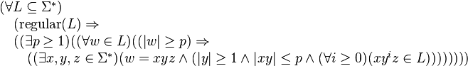
Specifically, the pumping lemma says that for any regular language L there exists a constant p such that any word w in L with length at least p can be split into three substrings, w = xyz, where the middle portion y must not be empty, such that the words xz, xyz, xyyz, xyyyz, … constructed by repeating y an arbitrary number of times (including zero times) are still in L. This process of repetition is known as "pumping". Moreover, the pumping lemma guarantees that the length of xy will be at most p, imposing a limit on the ways in which w may be split. Finite languages trivially satisfy the pumping lemma by having p equal to the maximum string length in L plus one.
The pumping lemma was first articulated by Y. Bar-Hillel, Micha A. Perles, Eli Shamir in 1961.[1] It is useful for disproving the regularity of a specific language in question. It is one of a few pumping lemmas, each with a similar purpose.
Below is a formal expression of the Pumping Lemma.
For example the language L = {anbn : n ≥ 0} over the alphabet Σ = {a, b} can be shown to be non-regular as follows. Let w, x, y, z, p, and i be as used in the formal statement for the pumping lemma above. Let w in L be given by w = apbp. By the pumping lemma, there must be some decomposition w = xyz with |xy| ≤ p and |y| ≥ 1 such that xyiz in L for every i ≥ 0. Using |xy| ≤ p, we know y only consists of instances of a. Moreover, because |y| ≥ 1, it contains at least one instance of the letter a. We now pump y up: xy2z has more instances of the letter a than the letter b, since we have added some instances of a without adding instances of b. Therefore xy2z is not in L. We have reached a contradiction. Therefore, the assumption that L is regular must be incorrect. Hence L is not regular.
The proof that the language of balanced (i.e., properly nested) parentheses is not regular follows the same idea. Given p, there is a string of balanced parentheses that begins with more than p left parentheses, so that y will consist entirely of left parentheses. By repeating y, we can produce a string that does not contain the same number of left and right parentheses, and so they cannot be balanced.
For example, the following image shows an FSA.

The FSA accepts the string: abcd. Since this string has a length which is at least as large as the number of states, which is four, the pigeonhole principle indicates that there must be at least one repeated state among the start state and the next four visited states. In this example, only q1 is a repeated state. Since the substring bc takes the machine through transitions that start at state q1 and end at state q1, that portion could be repeated and the FSA would still accept, giving the string abcbcd. Alternatively, the bc portion could be removed and the FSA would still accept giving the string ad. In terms of the pumping lemma, the string abcd is broken into an x portion a, a y portion bc and a z portion d.
For example, consider the language L = {uvwxy : u,y {0,1,2,3}*, v,w,x {0,1,2,3}∧(v=w∨v=x∨x=w)}
  {w : w {0,1,2,3}* and precisely 1/7 of the characters in w are 3's}. In other words, L
contains all strings over the alphabet {0,1,2,3} with a substring of
length 3 including a duplicate character, as well as all strings over
this alphabet where precisely 1/7 of the string's characters are 3's.
This language is not regular but can still be "pumped" with p = 5. Suppose some string s
has length at least 5. Then, since the alphabet has only four
characters, at least two of the five characters in the string must be
duplicates. They are separated by at most three characters.
{w : w {0,1,2,3}* and precisely 1/7 of the characters in w are 3's}. In other words, L
contains all strings over the alphabet {0,1,2,3} with a substring of
length 3 including a duplicate character, as well as all strings over
this alphabet where precisely 1/7 of the string's characters are 3's.
This language is not regular but can still be "pumped" with p = 5. Suppose some string s
has length at least 5. Then, since the alphabet has only four
characters, at least two of the five characters in the string must be
duplicates. They are separated by at most three characters.
www.cs.ucf.edu/courses/cot5310/Notes/COT5310Notes.ppt
notations as used in programming or markup languages. Recursion is the essential feature that distinguish CFGs
and CFLs from FAs and regular languages. Properties, strengths and weaknesses of CFLs. Equivalence of
CFGs and NPDAs. Non-equivalence of deterministic and non-deterministic PDAs. Parsing. Context sensitive
grammars CSG.
5.1 Context free grammars and languages (CFG, CFL)
Algol 60 pioneered CFGs and CFLs to define the syntax of programming languages (Backus-Naur Form).
Ex: arithmetic expression E, term T, factor F, primary P, a-op A = {+, -}, m-op M = {•, /}, exp-op = ^.
E -> T | EAT | AT, T -> F | TMF, F -> P | F^P,
P -> unsigned number | variable | function designator | ( E ) [Notice the recursion: E ->* ( E ) ]
Ex Recursive data structures and their traversals:
Binary tree T, leaf L, node N: T -> L | N T T (prefix) or T -> L | T N T (infix) or T -> L | T T N (suffix).
These definitions can be turned directly into recursive traversal procedures, e.g:
procedure traverse (p: ptr); begin if p ≠ nil then begin visit(p); traverse(p.left); traverse(p.right); end; end;
Df CFG: G = (V, A, P, S)
V: non-terminal symbols, “variables”; A: terminal symbols; S ∈ V: start symbol, “sentence”;
P: set of productions or rewriting rules of the form X -> w, where X ∈ V, w ∈ (V ∪ A)*
Rewriting step: for u, v, x, y, y’, z ∈ (V ∪ A)*: u -> v iff u = xyz, v = xy’z and y -> y’ ∈ P.
Derivation: “->*” is the transitive, reflexive closure of “->”, i.e.
u ->* v iff ∃ w0, w1, .. , wk with k ≥ 0 and u = w0, wj-1 -> wj, wk = v.
L(G) context free language generated by G: L(G) = {w ∈ A* | S ->* w }.
Ex Symmetric structures: L = { 0n 1n | n ≥ 0 }, or even palindromes L0 = { w wreversed | w ∈ {0, 1}* }
G(L) = ( {S}, {0, 1}, { S -> 0S1, S -> ε}, S ); G(L0) = ( {S}, {0, 1}, { S -> 0S0, S -> 1S1, S -> ε}, S )
Palindromes (length even or odd): L1 = {w | w = wreversed }. G(L1): add the rules: S -> 0, S -> 1 to G(L0).
Ex Parenthesis expressions: V = {S}, T = { (, ), [, ] }, P = { S -> ε, S -> (S), S -> [S], S -> SS }
Sample derivation: S -> SS -> SSS ->* ()[S][ ] -> ()[SS][ ] ->* ()[()[ ]][ ]
The rule S -> SS makes this grammar ambiguous. Ambiguity is undesirable in practice, since the syntactic
structure is generally used to convey semantic information.
S
S
S S
S
( ) ( ) ( ) ( ) ( ) ( )
S
S
S
S
≠ S
Ex Ambiguous structures in natural languages:
“Time flies like an arrow” vs. “Fruit flies like a banana”.
“Der Gefangene floh” vs. “Der gefangene Floh”.
Bad news: There exist CFLs that are inherently ambiguous, i.e. every grammar for them is ambiguous (see
Exercise). Moreover, the problem of deciding whether a given CFG G is ambiguous or not, is undecidable.
Good news: For practical purposes it is easy to design unambiguous CFG’s.
Exercise:
a) For the Algol 60 grammar G (simple arithmetic expressions) above, explain the purpose of the rule E -> AT
and show examples of its use. Prove or disprove: G is unambiguous.
b) Construct an unambiguous grammar for the language of parenthesis expressions above.
c) The ambiguity of the “dangling else”. Several programming languages (e.g. Pascal) assign to nested
if-then[-else] statements an ambiguous structure. It is then left to the semantics of the language to disambiguate.
Let E denote Boolean expression, S statement, and consider the 2 rules:
S -> if E then S, and S -> if E then S else S. Discuss the trouble with this grammar, and fix it.
d) Give a CFG for L = { 0i 1j 2k | i = j or j = k }. Try to prove: L is inherently ambiguous.
5.2 Equivalence of CFGs and NPDAs
Thm (CFG ~ NPDA): L ⊆ A* is CF iff ∃ NPDA M that accepts L.
Pf ->: Given CFL L, consider any grammar G(L) for L. Construct NPDA M that simulates all possible
derivations of G. M is essentially a single-state FSM, with a state q that applies one of G’s rules at a time. The
start state q0 initializes the stack with the content S ¢, where S is the start symbol of G, and ¢ is the bottom of
stack symbol. This initial stack content means that M aims to read an input that is an instance of S. In general, the
current stack content is a sequence of symbols that represent tasks to be accomplished in the characteristic LIFO
order (last-in first-out). The task on top of the stack, say a non-terminal X, calls for the next characters of the
imput string to be an instance of X. When these characters have been read and verified to be an instance of X, X
is popped from the stack, and the new task on top of the stack is started. When ¢ is on top of the stack, i.e. the
stack is empty, all tasks generated by the first instance of S have been successfully met, i.e. the input string read
so far is an instance of S. M moves to the accept state and stops.
The following transitions lead from q to q:
1) ε, X-> w for each rule X -> w. When X is on top of the stack, replace X by a right-hand side for X.
2) a, a -> ε for each a ∈ A. When terminal a is read as input and a is also on top of the stack, pop the stack.
Rule 1 reflects the following fact: one way to meet the task of finding an instance of X as a prefix of the input
string not yet read, is to solve all the tasks, in the correct order, present in the right-hand side w of the production
X -> w. M can be considered to be a non-deterministic parser for G. A formal proof that M accepts precisely L
can be done by induction on the length of the derivation of any w ∈ L. QED
Ex L = palindromes: G(L) = ( {S}, {0, 1}, { S -> 0S0, S -> 1S1, S -> 0, S -> 1, S -> ε}, S )
q0 q qf
ε, ε -> S ¢
Rule 2: 0, 0 -> ε 1, 1 -> ε
Rule 1:
ε, S -> 0 S0 ε, S -> 1 S1
ε, S -> 0 ε, S -> 1 ε, S -> ε
When q, q' are shown
explicitly, the transition:
(q, a, b) -> (q', v), v ∈ B*
is abbreviated as: a, b -> v
ε, ¢ -> ε
Pf <- (sketch): Given NPDA M, construct CFG G that generates L(M).
For simplicity’s sake, transform M to have the following features: 1) a single accept state, 2) empty stack before
accepting, and 3) each transition either pushes a single symbol, or pops a single symbol, but not both.
For each pair of states p, q ∈ Q, introduce non-terminal Vpq. L( Vpq ) = { w | Vpq ->* w } will be the language
of all strings that that can be derived from Vpq according to the productions of the grammar G to be constructed.
In particular, L( Vsf ) = L(M), where s is the starting state and f the accepting state of M.
Invariant:
Vpq generates all strings w that take M from p with an empty stack to q with an empty stack.
The idea is to relate all Vpq to each other in a way that reflects how labeled paths and subpaths through M’s state
space relate to each other. LIFO stack access implies: any w ∈ Vpq will lead M from p to q regardless of the
stack content at p, and leave the stack at q in the same condition as it was at p. Different w’s ∈ L( Vpq) may do
this in different ways, which leads to different rules of G:
1) The stack may be empty only in p and in q, never in between. If so, w = a v b, for some a, b ∈A, v ∈ A*. And
M includes the transitions (p, a, ε) -> (r, t) and (s,b, t) -> (q, ε). Add the rules: Vpq -> a Vrs b
2) The stack may be empty at some point between p and in q, in state r.
For each triple p, q, r ∈ Q, add the rules: Vpq -> Vpr Vrq.
3) For each p ∈ Q, add the rule Vpp -> ε .
The figure at left illustrates Rule1, at right Rule 2. If M includes the transitions (p, a, ε) -> (r, t) and (s,b, t) -> (q,
ε), then one way to lead M from p to q with identical stack content at the start and the end of the journey is to
break the trip into three successive parts: 1) to read a symbol ‘a’ and push ‘t’; 2) travel from r to s with identical
stack content at the start and the end of this sub-journey; 3) to read a symbol ‘b’ and pop ‘t’.
p q
r s
Vpq
Vrs
a, ε -> t b, t -> ε
t t q
p
r
Vpq
Vpr
Vrq
5.3 Normal forms
When trying to prove that all objects in some class C have a given property P, it is often useful to first prove that
each object O in C can be transformed to some equivalent object O’ in some subclass C’ of C. Here,
‘equivalent’ implies that the transformation preserves the property P of interest. Thereafter, the argument can be
limited to the the subclass C’, taking advantage of any additional properties this subclass may have.
Any CFG can be transformed into a number of “normal forms” (NF) that are (almost!) equivalent. Here,
‘equivalent’ means that the two grammars define the same language, and the proviso “almost” is necessary
because these normal forms cannot generate the null string.
Chomsky normal form (right-hand sides are short):
All rules are of the form X -> Y Z or X -> a, for some non-terminals X, Y, Z ∈ V and terminal a ∈ A
Thm: Every CFG G can be transformed into a Chomsky NF G’ such that L(G’) = L(G) - {ε}.
Pf idea: repeatedly replace a rule X -> v w, |v| ≥ 1, |w| ≥ 2 by X -> Y Z, Y -> v, Z -> w, where Y and Z are new
non-terminals used only in these new rules. Both right hand sides v and w are shorter than the original right hand
side v w.
The Chomsky NF changes the syntactic structure of L(G), an undesirable side effect in practice. But Chomsky
NF turns all syntactic structures into binary trees, a useful technical device that we exploit in later sections on the
Pumping Lemma and the CYK parsing algorithm.
Greibach normal form (at every step, produce 1 terminal symbol at the far left - useful for parsing):
All rules are of the form X -> a w, for some terminal a ∈ A, and some w ∈ V*
Thm: Every CFG G can be transformed into a Greibach NF G’ such that L(G’) = L(G) - {ε}.
Pf idea: for a rule X -> Y w, ask whether Y can ever produce a terminal at the far left, i.e. Y ->* a v. If so, replace
X -> Y w by rules such as X -> a v w. If not, X -> Y w can be omitted, as it will never lead to a terminating
derivation.
5.4 The pumping lemma for CFLs
Recall the pumping lemma for regular languages, a mathematically precise statement of the intuitive notion “a
FSM can count at most up to some constant n”. It says that for any regular language L, any sufficiently long
word w in L can be split into 3 parts, w = x y z, such that all strings x yk z, for any k ≥ 0, are also in L.
PDAs, which correspond to CFGs, can count arbitrarily high - though essentially in unary notation, i.e. by
storing k symbols to represent the number k. But the LIFO access limitation implies that the stack can only be
used to represent one single independent counter at a time. To understand what ‘independent’ means, consider a
PDA that recognizes a language of balanced parenthesis expressions, such as ((([[..]]))). This task clearly calls
for an arbitrary number of counters to be stored at the same time, each one dedicated to counting his own
subexpression. In the example above, the counter for ‘(((‘ must be saved when the counter for ‘[[‘ is activated.
Fortunately, balanced parentheses are nested in such a way that changing from one counter to another matches
the LIFO access pattern of a stack - when a counter, run down to 0, is no longer needed, the next counter on top
of the stack is exactly the next one to be activated. Thus, the many counters coded into the stack interact in a
controlled manner, they are not independent.
The pumping lemma for CFLs is a precise statement of this limitation. It asserts that every long word in L serves
as a seed that generates an infinity of related words that are also in L.
Thm: For every CFL L there is a constant n such that every z ∈ L of length |z| ≥ n can be written as
z = u v w x y such that the following holds:
1) v x ≠ ε , 2) |v w x| ≤ n, and 3) u vk w xk y ∈ L for all k ≥ 0.
Pf: Given CFL L, choose any G = G(L) in Chomsky NF. This implies that the parse tree of any z ∈ L is a
binary tree, as shown in the figure below at left. The length n of the string at the leaves and the height h of a
binary tree are related by h ≥ log n, i.e. a long string requires a tall parse tree. By choosing the critical length
n = 2 |V | + 1 we force the height of the parse trees considered to be h ≥ |V| + 1. On a root-to-leaf path of
length ≥ |V| + 1 we encounter at least |V| + 1 nodes labeled by non-terminals. Since G has only |V| distinct
non-terminals, this implies that on some long root-to-leaf path we must encounter 2 nodes labeled with the same
non-terminal, say W, as shown at right.
a
S
A
B C
D
F
E
c
d
b u v w x y
≥ |V| + 1 ≤ |V| + 1
W
W
S
For two such occurrences of W (in particular, the two lowest ones), and for some u, v, y, x, w ∈ A*, we have: S -
>* u W y, W ->* v W x and W ->* w. But then we also have W ->* v2 W x2, and in general, W ->* vk W
xk, and S ->* u vk W xk y and S ->* u vk w xk y for all k ≥ 0, QED.
For problems where intuition tells us“a PDA can’t do that”, the pumping lemma is often the perfect tool needed
to prove rigorously that a language is not CF. For example, intuition suggests that neither of the languages L1 =
{ 0k 1k 2k / k ≥ 0 } or L2 = { w w / w ∈ {0, 1} } is recognizable by some PDA.
For L1, a PDA would have to count up the 0s, then count down the 1s to make sure there are equally many 0s
and 1s. Thereafter, the counters is zero, and although we can count the 2s, can’t compare that number to the
number of 0s, or of 1s, an information that is now lost.
For L2, a PDA would have to store the first half of the input, namely w, and compare that to the second half to
verify that the latter is also w. Whereas this worked trivially for palindromes, w wreversed, the order w w is the
worst case possible for LIFO access: although the stack contains all the information needed, we can’t extract the
info we need at the time we need it. The pumping lemma confirms these intuitive judgements.
Ex 1: L1 = { 0k 1k 2k / k ≥ 0 } is not context free.
Pf (by contradiction): Assume L is CF, let n be the constant asserted by the pumping lemma.
Consider z = 0n 1n 2n = u v w x y. Although we don’t know where vwx is positioned within z, the assertion |v
w x| ≤ n implies that v w x contains at most two distinct letters among 0, 1, 2. In other words, one or two of the
three letters 0, 1, 2 is missing in vwx. Now consider u v2 w x2 y. By the pumping lemma, it must be in L. The
assertion |v x| ≥ 1 implies that u v2 w x2 y is longer than u v w x y. But u v w x y had an equal number of 0s, 1s,
and 2s, whereas u v2 w x2 y cannot, since only one or two of the three distinct symbols increased in number. This
contradiction proves the thm.
Ex 2: L2 = { w w / w ∈ {0, 1} } is not context free.
Pf (by contradiction): Assume L is CF, let n be the constant asserted by the pumping lemma.
Consider z = 0n+1 1n+1 0n+1 1n+1 = u v w x y. Using k = 0, the lemma asserts z0 = u w y ∈ L, but we show
that z0 cannot have the form t t, for any string t, and thus that z0 ∉ L, leading to a contradiction. Recall that |v w
x| ≤ n, and thus, when we delete v and x, we delete symbols that are within a distance of at most n from each
other. By analyzing three cases we show that, under this restriction, it is impossible to delete symbols in such a
way as to retain the property that the shortened string z0 = u w x has the form t t. We illustrate this using the
example n = 3, but the argument holds for any n.
Given z = 0 0 0 0 1 1 1 1 0 0 0 0 1 1 1 1, slide a window of length n = 3 across z, and delete any characters you
want from within the window. Observe that the blocks of 0s and of 1s within z are so long that the truncated z,
call it z’, still has the form “0s 1s 0s 1s”. This implies that if z’ can be written as z’ = t t, then t must have the
form t = “0s 1s”. Checking the three cases: the window of length 3 lies entirely within the left half of z; the
window straddles the center of z; and the window lies entirely within the right half of z, we observe that in none
of these cases z’ has the form z’ = t t, and thus that z0 = u w y ∉ L. QED
5.5 Closure properties of the class of CFLs
Thm (CFL closure properties): The class of CFLs over an alphabet A is closed under the regular operations
union, catenation, and Kleene star.
Pf: Given CFLs L, L’ ⊆ A*, consider any grammars G, G’ that generate L and L’, respectively. Combine G and
G’ appropriately to obtain grammars for L ∪ L’, L L’, and L*. E.g, if G = (V, A, P, S), we obtain
G(L*) = ( V ∪ {S0}, A, P ∪ { S0 -> S S0 , S0 -> ε }, S0 ).
The proof above is analogous to the proof of closure of the class or regular languages under union, catenation,
and Kleene star. There we combined two FAs into a single one using series, parallel, and loop combinations of
FAs. But beyond the three regular operations, the analogy stops. For regular languages, we proved closure under
complement by appealing to deterministic FAs as acceptors. For these, changing all accepting states to nonaccepting,
and vice versa, yields the complement of the language accepted. This reasoning fails for CFL’s,
because deterministic PDAs accept only a subclass of CFLs. For non-deterministic PDAs, changing accepting
states to non-accepting, and vice versa, does not produce the complement of the language accepted. Indeed,
closure under complement does not hold for CFLs.
Thm: The class of CFLs over an alphabet A
is not closed under intersection and is not closed under omplement.
We prove this theorem in two ways: first, by exhibiting two CFLs whose intersection is provably not CF, and
second, by exhibiting a CFL whose complement is provably not CF.
Pf ∩: Consider CFLs L0 = { 0m 1m 2n | m, n ≥ 1 } and L1 = { 0m 1n 2n | m, n ≥ 1 }.
L0 ∩ L1 = { 0k 1k 2k | k ≥ 1 } is not CF, as we proved in the previous section using the pumping lemma.
This implies that the class of CFLs is not closed under complement. If it were, it would also be closed under
intersection, because of the identity: L ∩ L’ = ¬(¬L ∪ ¬L’ ). But we also prove this result in a direct way
by exhibiting a CFL L whose complement is not context free. L’s complement is the notorious language L2 =
{ w w / w ∈ {0, 1} } , which we have proven not context free using the pumping lemma.
Pf ¬: We show that L = { u | u is not of the form u = w w } is context free by exhibiting a CFG for L:
S -> Y | Z | Y Z | Z Y
Y -> 1 | 0 Y 0 | 0 Y 1 | 1 Y 0 | 1 Y 1
Z -> 0 | 0 Z 0 | 0 Z 1 | 1 Z 0 | 1 Z 1
The productions for Y generate all odd strings, i.e. strings of odd length, with a 1 as its center symbol.
Analogously, Z generates all odd strings with a 0 as its center symbol. Odd strings are not of the form
u = w w, hence they are included in L by the productions S -> Y | Z . Now we show that the strings u of even
length that are not of the form u = w w are precisely those of the form Y Z or Z Y.
First, consider a word of the form Y Z, such as the catenation of y = 1 1 0 1 0 0 0 and z = 1 0 1, where the center
1 of y and the center 0 of z are highlighted. Writing y z = 1 1 0 1 0 0 0 1 0 1 as the catenation of two strings of
equal length, namely 1 1 0 1 0 and 0 0 1 0 1, shows that the former center symbols 1 of y and 0 of z have both
become the 4-th symbol in their respective strings of length 5. Thus, they are a witness pair whose clash shows
that y z ≠ w w for any w. This, and the analogous case for Z Y, show that the set of strings of the form Y Z or Z Y
are in L.
Conversely, consider any even word u = a1 a2 .. aj .. ak b1 b2 .. bj .. bk which is not of the form u = w w. There
exists an index j where aj ≠ bj, and we can take each of aj and bj as center symbol of its own odd string. The
following example shows a clashing pair at index j = 4: u = 1 1 0 0 1 1 1 0 1 1.
Now u = 1 1 0 0 1 1 1 0 1 1 can be written as u = z y, where z = 1 1 0 0 1 1 1 ∈ Z and y = 0 1 1 ∈ Y.
The following figure how the various string lengths labeled α and β add up.
a1 a2 .. . . aj .. ak b1 b2 .. . . bj .. bk
α β α β
α α β β
symmetry axis
odd string with center symbol aj odd string
5.6 The “word problem”. CFL parsing in time O(n3) by means of dynamic programming
Informally, the word problem asks: given G and w ∈ A*, decide whether w ∈ L(G).
More precisely: is there an algorithm that applies to any grammar G in some given class of grammars, and any w
∈ A*, to decide whether w ∈ L(G)?
Many algorithms solve the word problem for CFGs, e.g: a) convert G to Greibach NF and enumerate all
derivations of length ≤ |w| to see whether any of them generates w; or b) construct an NPDA M that accepts
L(G), and feed w into M.
Ex1: L = { 0k 1k | k ≥ 1 }. G: S -> 01 | 0 S1. Use “0” as a stack symbol to count the number of 0s.
0, ε -> 0 q0 q1
1, 0 -> ε
1, 0 -> ε Accept on
empty stack
Ex2: L = {w ∈ {0, 1}* | #0s = #1s }. G: S -> ε | 0 Y’ | 1 Z’, Y’ -> 1 S | 0 Y’ Y’, Z’ -> 0 S | 1 Z’ Z’
Invariant: Y’ generates any string with an extra 1, Z’ generates any string with an extra 0.
The production Z’ -> 0 S | 1 Z’ Z’ means that Z’ has two ways to meet its goal: either produce a 0 now and
follow up with a string in S, i.e with an equal number of 0s and 1s; or produce a 1 but create two new tasks Z’.
1, ε -> 1
ε, ¢ -> ε
#0s = #1s
#0s > #1s ε, ¢ -> ε #0s < #1s
0, ε -> 0
1, 0 -> ε 0, 1 -> ε
For CFGs there is a “bottom up” algorithm (Cocke, Younger, Kasami) that systematically computes all possible
parse trees of all contiguous substrings of the string w to be parsed, and works in time O( |w|3 ). We illustrate the
idea of the CYK algorithm using the following example:
Ex2a: L = {w ∈ {0, 1 }+ | #0s = #1s }. G: S -> 0 Y’ | 1 Z’, Y’ -> 1S | 0 Y’ Y’, Z’ -> 0 S | 1 Z’ Z’
We exclude the nullstring in order to convert G to Chomsky NF. For the sake of formality, introduce Y that
generates a single 1, similarly for Z and 0. Shorten the right hand side 0 Z’ Z’ by introducing a non terminal Z”
-> Z’ Z’, and similarly Y” -> Y’Y’. Every w ∈ Z” can be written as w = u v, u ∈ Z’, v ∈ Z’. As we read w
from left to write, there comes an index k where #1s = #0s +1, and that prefix of w can be taken as u. The
remainder v has again #1s = #0s +1.
The grammar below maintains the invariants: Y generates a single “1”; Y’ generates any string with an extra
“1”; Y” generates any string with 2 extra “1”. Analogously for Z, Z’, Z” and “0”.
S -> Z Y’ | Y Z’ start with a 0 and remember to generate an extra 1, or start with a 1 and ...
Z -> 0, Y -> 1 Z and Y are mere formalities
Z’ -> 0 | Z S | Y Z” produce an extra 0 now, or produce a 1 and remember to generate 2 extra 0s
Y’ -> 1 | Y S | Z Y” produce an extra 1 now, or produce a 0 and remember to generate 2 extra 1s
Z” -> Z’ Z’, Y” -> Y’Y’ split the job of generating 2 extra 0s or 2 extra 1s
The following table parses a word w = 001101 with |w| = n. Each of the n (n+1)/2 entries corresponds to a
substring of w. Entry (L, i) records all the parse trees of the substring of length L that begins at index i. The
entries for L = 1 correspond to rules that produce a single terminal, the other entries to rules that produce 2 nonterminals.
0 1 1 0
Y" -> Y'Y'
Z -> 0
Z' -> 0
Z -> 0
Z' -> 0
Y -> 1
Y' -> 1
Y -> 1
Y' -> 1
S -> Z Y' S -> Y Z'
Y' -> Z Y" Y' -> Y S
S -> Z Y'
3 attempts
to prove
S ->* 0 1 1 0
0 0 1 1 0 1
1
2
3
4
5
6
L w =
Y" -> Y'Y'
Y" -> Y'Y'
Z -> 0
Z' -> 0
Z -> 0
Z' -> 0
Z -> 0
Z' -> 0
Y -> 1
Y' -> 1
Y -> 1
Y' -> 1
Y -> 1
Y' -> 1
Z" -> Z' Z' S -> Z Y' S -> Y Z' S -> ZY'
Z' -> Z S Y' -> Z Y" Y' -> Y S Y' -> Y S
S -> Z Y' S -> Z Y'
Z" -> Z S Y' -> Z Y"
S -> Z Y'
Notice the framed rule
Y" -> Y' Y'
matches in 2 distinct ways
(ambiguous grammar)
The picture at the lower right shows that for each entry at level L, we must try (L-1) distinct ways of splitting that
entry’s substring into 2 parts. Since (L-1) < n and there are n (n+1)/2 entries to compute, the CYK parser works
in time O(n3).
Useful CFLs, such as parts of programming languages, should be designed so as to admit more efficient parsers,
preferably parsers that work in linear time. LR(k) grammars and languages are a subset of CFGs and CFLs that
can be parsed in a single scan from left to right, with a look-ahead of k symbols.
5.7 Context sensitive grammars and languages
The rewriting rules B -> w of a CFG imply that a non-terminal B can be replaced by a word w ∈ (V ∪ A)* “in
any context”. In contrast, a context sensitive grammar (CSG) has rules of the form:
u B v -> u w v, where u, v, w ∈ (V ∪ A)*,
implying that B can be replaced by w only in the context “u on the left, v on the right”.
It turns out that this definition is equivalent (apart from the nullstring ε) to requiring that any CSG rule be of the
form v -> w, where v, w ∈ (V ∪ A)*, and |v| ≤ |w|. This monotonicity property (in any derivation, the current
string never gets shorter) implies that the word problem for CSLs: “given CSG G and given w, is w ∈ L(G)?”
is decidable. An exhaustive enumeration of all derivations up to the length |w| settles the issue.
As an example of the greater power of CSGs over CFGs, recall that we used the pumping lemma to prove that the
language 0k 1k 2k is not CF. By way of contrast, we prove:
Thm: L = { 0k 1k 2k / k ≥ 1 } is context sensitive.
The following CSG generates L. Function of the non-terminals V = {S, B, C, Y, Z}: each Y and Z generates a 1
or a 0 at the proper time; B initially marks the beginning (left end) of the string, and later converts the Zs into 0s;
C is a counter that ensures an equal number of 0s, 1s, 2s are generated. Non-terminals play a similar role as
markers in Markov algorithms. Whereas the latter have a deterministic control structure, grammars are nondeterministic.
S -> B K 2 at the last step in any derivation, B K generates 01, balancing this ‘2’
K -> Z Y K 2 counter K generates (ZY)k 2k
K -> C when k has been fixed, C may start converting Ys into 1s
Y Z -> Z Y Zs may move towards the left, Ys towards the right at any time
B Z -> 0 B B may convert a Z into a 0 and shift it left at any time
Y C -> C 1 C may convert a Y into a 1 and shift it right at any time
B C -> 01 when B and C meet, all permutations, shifts and conversions have been done
Hw 5.1: Context-free grammars and pushdown automata
Consider the context-free grammar G with non-terminals S and P, start symbol S, terminals ‘(‘, ‘)’ and ‘0’, and
productions: S -> S P | ε ; P -> ( S ) | 0 .
a) Draw a derivation tree for each of the 4 shortest strings produced by G.
b) Prove or disprove: the grammar G is unambiguous.
c) Design a pushdown automaton M to accept the language L(G). Let M be deterministic if possible,
or non-deterministic if necessary.
Ex: Show that L = {ww | w ∈ {0, 1}* } is context sensitive.
Ex: Recall the grammar G1 of arithmetic expressions, e.g. in the simplified form:
E -> T | EAT, T -> F | TMF, F -> N | V | ( E ) , A -> + | - , M -> * | /
For simplicity’s sake, we limit numbers to single bits, i.e. N -> 0 | 1, and use only 3 variables, V -> x | y | z
a) Extend G1 to a grammar G2 that includes function terms, such as f(x) and g( 1 - x/y)
Use only 3 function symbols defined in a new production H -> f | g | h
b) Extend G2 to a grammar G3 that includes integration terms, such as S [ a, b ] f(x) dx, a linearized form of
“integral from a to b of f(x) dx”.
c) Discuss the strengths and weaknesses of CFGs as tools to solve the tasks a) and b).
Ex: Let L = {ww | w ∈ {0, 1}* }
a) Prove that L is not context free, and b) prove that L is context sensitive.
Useful Links for Automata
http://www.cs.uky.edu/~lewis/texts/theory/automata/pd-auto.pdf
http://www.eecs.wsu.edu/~ananth/CptS317/Lectures/IntroToAutomataTheory.pdf
Pumping lemma for regular languages
From Wikipedia, the free encyclopedia
In the theory of formal languages, the pumping lemma for regular languages describes an essential property of all regular languages. Informally, it says that all sufficiently long words in a regular language may be pumped
— that is, have a middle section of the word repeated an arbitrary
number of times — to produce a new word which also lies within the same
language.Specifically, the pumping lemma says that for any regular language L there exists a constant p such that any word w in L with length at least p can be split into three substrings, w = xyz, where the middle portion y must not be empty, such that the words xz, xyz, xyyz, xyyyz, … constructed by repeating y an arbitrary number of times (including zero times) are still in L. This process of repetition is known as "pumping". Moreover, the pumping lemma guarantees that the length of xy will be at most p, imposing a limit on the ways in which w may be split. Finite languages trivially satisfy the pumping lemma by having p equal to the maximum string length in L plus one.
The pumping lemma was first articulated by Y. Bar-Hillel, Micha A. Perles, Eli Shamir in 1961.[1] It is useful for disproving the regularity of a specific language in question. It is one of a few pumping lemmas, each with a similar purpose.
Contents[hide] |
[edit] Formal statement
Let L be a regular language. Then there exists an integer p ≥ 1 depending only on L such that every string w in L of length at least p (p is called the "pumping length") can be written as w = xyz (i.e., w can be divided into three substrings), satisfying the following conditions:- |y| ≥ 1
- |xy| ≤ p
- for all i ≥ 0, xyiz ∈ L
Below is a formal expression of the Pumping Lemma.
[edit] Use of lemma
The pumping lemma is often used to prove that a particular language is non-regular: a proof by contradiction (of the language's regularity) may consist of exhibiting a word (of the required length) in the language which lacks the property outlined in the pumping lemma.For example the language L = {anbn : n ≥ 0} over the alphabet Σ = {a, b} can be shown to be non-regular as follows. Let w, x, y, z, p, and i be as used in the formal statement for the pumping lemma above. Let w in L be given by w = apbp. By the pumping lemma, there must be some decomposition w = xyz with |xy| ≤ p and |y| ≥ 1 such that xyiz in L for every i ≥ 0. Using |xy| ≤ p, we know y only consists of instances of a. Moreover, because |y| ≥ 1, it contains at least one instance of the letter a. We now pump y up: xy2z has more instances of the letter a than the letter b, since we have added some instances of a without adding instances of b. Therefore xy2z is not in L. We have reached a contradiction. Therefore, the assumption that L is regular must be incorrect. Hence L is not regular.
The proof that the language of balanced (i.e., properly nested) parentheses is not regular follows the same idea. Given p, there is a string of balanced parentheses that begins with more than p left parentheses, so that y will consist entirely of left parentheses. By repeating y, we can produce a string that does not contain the same number of left and right parentheses, and so they cannot be balanced.
[edit] Proof of the pumping lemma
For every regular language there is a finite state automaton (FSA) that accepts the language. The number of states in such an FSA are counted and that count is used as the pumping length p. For a string of length at least p, let s0 be the start state and let s1, ..., sp be the sequence of the next p states visited as the string is emitted. Because the FSA has only p states, within this sequence of p + 1 visited states there must be at least one state that is repeated. Write S for such a state. The transitions that take the machine from the first encounter of state S to the second encounter of state S match some string. This string is called y in the lemma, and since the machine will match a string without the y portion, or the string y can be repeated any number of times, the conditions of the lemma are satisfied.For example, the following image shows an FSA.

The FSA accepts the string: abcd. Since this string has a length which is at least as large as the number of states, which is four, the pigeonhole principle indicates that there must be at least one repeated state among the start state and the next four visited states. In this example, only q1 is a repeated state. Since the substring bc takes the machine through transitions that start at state q1 and end at state q1, that portion could be repeated and the FSA would still accept, giving the string abcbcd. Alternatively, the bc portion could be removed and the FSA would still accept giving the string ad. In terms of the pumping lemma, the string abcd is broken into an x portion a, a y portion bc and a z portion d.
[edit] General version of pumping lemma for regular languages
If a language L is regular, then there exists a number p ≥ 1 (the pumping length) such that every string uwv in L with |w| ≥ p can be written in the form- uwv = uxyzv
- uxyizv is in L for every integer i ≥ 0.[2]
[edit] Converse of lemma not true
Note that while the pumping lemma states that all regular languages satisfy the conditions described above, the converse of this statement is not true: a language that satisfies these conditions may still be non-regular. In other words, both the original and the general version of the pumping lemma give a necessary but not sufficient condition for a language to be regular.For example, consider the language L = {uvwxy : u,y
{0,1,2,3}*, v,w,x {0,1,2,3}∧(v=w∨v=x∨x=w)} {w : w {0,1,2,3}* and precisely 1/7 of the characters in w are 3's}. In other words, L
contains all strings over the alphabet {0,1,2,3} with a substring of
length 3 including a duplicate character, as well as all strings over
this alphabet where precisely 1/7 of the string's characters are 3's.
This language is not regular but can still be "pumped" with p = 5. Suppose some string s
has length at least 5. Then, since the alphabet has only four
characters, at least two of the five characters in the string must be
duplicates. They are separated by at most three characters.- If the duplicate characters are separated by 0 characters, or 1, pump one of the other two characters in the string, which will not affect the substring containing the duplicates.
- If the duplicate characters are separated by 2 or 3 characters, pump 2 of the characters separating them. Pumping either down or up results in the creation of a substring of size 3 that contains 2 duplicate characters.
- The second condition of L ensures that L is not regular: i.e., there are an infinite number of strings that are in L but cannot be obtained by pumping some smaller string in L.
www.cs.ucf.edu/courses/cot5310/Notes/COT5310Notes.ppt
Context free grammars (CFG) and languages (CFL)
Goals of this chapter: CFGs and CFLs as models of computation that define the syntax of hierarchical formalnotations as used in programming or markup languages. Recursion is the essential feature that distinguish CFGs
and CFLs from FAs and regular languages. Properties, strengths and weaknesses of CFLs. Equivalence of
CFGs and NPDAs. Non-equivalence of deterministic and non-deterministic PDAs. Parsing. Context sensitive
grammars CSG.
5.1 Context free grammars and languages (CFG, CFL)
Algol 60 pioneered CFGs and CFLs to define the syntax of programming languages (Backus-Naur Form).
Ex: arithmetic expression E, term T, factor F, primary P, a-op A = {+, -}, m-op M = {•, /}, exp-op = ^.
E -> T | EAT | AT, T -> F | TMF, F -> P | F^P,
P -> unsigned number | variable | function designator | ( E ) [Notice the recursion: E ->* ( E ) ]
Ex Recursive data structures and their traversals:
Binary tree T, leaf L, node N: T -> L | N T T (prefix) or T -> L | T N T (infix) or T -> L | T T N (suffix).
These definitions can be turned directly into recursive traversal procedures, e.g:
procedure traverse (p: ptr); begin if p ≠ nil then begin visit(p); traverse(p.left); traverse(p.right); end; end;
Df CFG: G = (V, A, P, S)
V: non-terminal symbols, “variables”; A: terminal symbols; S ∈ V: start symbol, “sentence”;
P: set of productions or rewriting rules of the form X -> w, where X ∈ V, w ∈ (V ∪ A)*
Rewriting step: for u, v, x, y, y’, z ∈ (V ∪ A)*: u -> v iff u = xyz, v = xy’z and y -> y’ ∈ P.
Derivation: “->*” is the transitive, reflexive closure of “->”, i.e.
u ->* v iff ∃ w0, w1, .. , wk with k ≥ 0 and u = w0, wj-1 -> wj, wk = v.
L(G) context free language generated by G: L(G) = {w ∈ A* | S ->* w }.
Ex Symmetric structures: L = { 0n 1n | n ≥ 0 }, or even palindromes L0 = { w wreversed | w ∈ {0, 1}* }
G(L) = ( {S}, {0, 1}, { S -> 0S1, S -> ε}, S ); G(L0) = ( {S}, {0, 1}, { S -> 0S0, S -> 1S1, S -> ε}, S )
Palindromes (length even or odd): L1 = {w | w = wreversed }. G(L1): add the rules: S -> 0, S -> 1 to G(L0).
Ex Parenthesis expressions: V = {S}, T = { (, ), [, ] }, P = { S -> ε, S -> (S), S -> [S], S -> SS }
Sample derivation: S -> SS -> SSS ->* ()[S][ ] -> ()[SS][ ] ->* ()[()[ ]][ ]
The rule S -> SS makes this grammar ambiguous. Ambiguity is undesirable in practice, since the syntactic
structure is generally used to convey semantic information.
S
S
S S
S
( ) ( ) ( ) ( ) ( ) ( )
S
S
S
S
≠ S
Ex Ambiguous structures in natural languages:
“Time flies like an arrow” vs. “Fruit flies like a banana”.
“Der Gefangene floh” vs. “Der gefangene Floh”.
Bad news: There exist CFLs that are inherently ambiguous, i.e. every grammar for them is ambiguous (see
Exercise). Moreover, the problem of deciding whether a given CFG G is ambiguous or not, is undecidable.
Good news: For practical purposes it is easy to design unambiguous CFG’s.
Exercise:
a) For the Algol 60 grammar G (simple arithmetic expressions) above, explain the purpose of the rule E -> AT
and show examples of its use. Prove or disprove: G is unambiguous.
b) Construct an unambiguous grammar for the language of parenthesis expressions above.
c) The ambiguity of the “dangling else”. Several programming languages (e.g. Pascal) assign to nested
if-then[-else] statements an ambiguous structure. It is then left to the semantics of the language to disambiguate.
Let E denote Boolean expression, S statement, and consider the 2 rules:
S -> if E then S, and S -> if E then S else S. Discuss the trouble with this grammar, and fix it.
d) Give a CFG for L = { 0i 1j 2k | i = j or j = k }. Try to prove: L is inherently ambiguous.
5.2 Equivalence of CFGs and NPDAs
Thm (CFG ~ NPDA): L ⊆ A* is CF iff ∃ NPDA M that accepts L.
Pf ->: Given CFL L, consider any grammar G(L) for L. Construct NPDA M that simulates all possible
derivations of G. M is essentially a single-state FSM, with a state q that applies one of G’s rules at a time. The
start state q0 initializes the stack with the content S ¢, where S is the start symbol of G, and ¢ is the bottom of
stack symbol. This initial stack content means that M aims to read an input that is an instance of S. In general, the
current stack content is a sequence of symbols that represent tasks to be accomplished in the characteristic LIFO
order (last-in first-out). The task on top of the stack, say a non-terminal X, calls for the next characters of the
imput string to be an instance of X. When these characters have been read and verified to be an instance of X, X
is popped from the stack, and the new task on top of the stack is started. When ¢ is on top of the stack, i.e. the
stack is empty, all tasks generated by the first instance of S have been successfully met, i.e. the input string read
so far is an instance of S. M moves to the accept state and stops.
The following transitions lead from q to q:
1) ε, X-> w for each rule X -> w. When X is on top of the stack, replace X by a right-hand side for X.
2) a, a -> ε for each a ∈ A. When terminal a is read as input and a is also on top of the stack, pop the stack.
Rule 1 reflects the following fact: one way to meet the task of finding an instance of X as a prefix of the input
string not yet read, is to solve all the tasks, in the correct order, present in the right-hand side w of the production
X -> w. M can be considered to be a non-deterministic parser for G. A formal proof that M accepts precisely L
can be done by induction on the length of the derivation of any w ∈ L. QED
Ex L = palindromes: G(L) = ( {S}, {0, 1}, { S -> 0S0, S -> 1S1, S -> 0, S -> 1, S -> ε}, S )
q0 q qf
ε, ε -> S ¢
Rule 2: 0, 0 -> ε 1, 1 -> ε
Rule 1:
ε, S -> 0 S0 ε, S -> 1 S1
ε, S -> 0 ε, S -> 1 ε, S -> ε
When q, q' are shown
explicitly, the transition:
(q, a, b) -> (q', v), v ∈ B*
is abbreviated as: a, b -> v
ε, ¢ -> ε
Pf <- (sketch): Given NPDA M, construct CFG G that generates L(M).
For simplicity’s sake, transform M to have the following features: 1) a single accept state, 2) empty stack before
accepting, and 3) each transition either pushes a single symbol, or pops a single symbol, but not both.
For each pair of states p, q ∈ Q, introduce non-terminal Vpq. L( Vpq ) = { w | Vpq ->* w } will be the language
of all strings that that can be derived from Vpq according to the productions of the grammar G to be constructed.
In particular, L( Vsf ) = L(M), where s is the starting state and f the accepting state of M.
Invariant:
Vpq generates all strings w that take M from p with an empty stack to q with an empty stack.
The idea is to relate all Vpq to each other in a way that reflects how labeled paths and subpaths through M’s state
space relate to each other. LIFO stack access implies: any w ∈ Vpq will lead M from p to q regardless of the
stack content at p, and leave the stack at q in the same condition as it was at p. Different w’s ∈ L( Vpq) may do
this in different ways, which leads to different rules of G:
1) The stack may be empty only in p and in q, never in between. If so, w = a v b, for some a, b ∈A, v ∈ A*. And
M includes the transitions (p, a, ε) -> (r, t) and (s,b, t) -> (q, ε). Add the rules: Vpq -> a Vrs b
2) The stack may be empty at some point between p and in q, in state r.
For each triple p, q, r ∈ Q, add the rules: Vpq -> Vpr Vrq.
3) For each p ∈ Q, add the rule Vpp -> ε .
The figure at left illustrates Rule1, at right Rule 2. If M includes the transitions (p, a, ε) -> (r, t) and (s,b, t) -> (q,
ε), then one way to lead M from p to q with identical stack content at the start and the end of the journey is to
break the trip into three successive parts: 1) to read a symbol ‘a’ and push ‘t’; 2) travel from r to s with identical
stack content at the start and the end of this sub-journey; 3) to read a symbol ‘b’ and pop ‘t’.
p q
r s
Vpq
Vrs
a, ε -> t b, t -> ε
t t q
p
r
Vpq
Vpr
Vrq
5.3 Normal forms
When trying to prove that all objects in some class C have a given property P, it is often useful to first prove that
each object O in C can be transformed to some equivalent object O’ in some subclass C’ of C. Here,
‘equivalent’ implies that the transformation preserves the property P of interest. Thereafter, the argument can be
limited to the the subclass C’, taking advantage of any additional properties this subclass may have.
Any CFG can be transformed into a number of “normal forms” (NF) that are (almost!) equivalent. Here,
‘equivalent’ means that the two grammars define the same language, and the proviso “almost” is necessary
because these normal forms cannot generate the null string.
Chomsky normal form (right-hand sides are short):
All rules are of the form X -> Y Z or X -> a, for some non-terminals X, Y, Z ∈ V and terminal a ∈ A
Thm: Every CFG G can be transformed into a Chomsky NF G’ such that L(G’) = L(G) - {ε}.
Pf idea: repeatedly replace a rule X -> v w, |v| ≥ 1, |w| ≥ 2 by X -> Y Z, Y -> v, Z -> w, where Y and Z are new
non-terminals used only in these new rules. Both right hand sides v and w are shorter than the original right hand
side v w.
The Chomsky NF changes the syntactic structure of L(G), an undesirable side effect in practice. But Chomsky
NF turns all syntactic structures into binary trees, a useful technical device that we exploit in later sections on the
Pumping Lemma and the CYK parsing algorithm.
Greibach normal form (at every step, produce 1 terminal symbol at the far left - useful for parsing):
All rules are of the form X -> a w, for some terminal a ∈ A, and some w ∈ V*
Thm: Every CFG G can be transformed into a Greibach NF G’ such that L(G’) = L(G) - {ε}.
Pf idea: for a rule X -> Y w, ask whether Y can ever produce a terminal at the far left, i.e. Y ->* a v. If so, replace
X -> Y w by rules such as X -> a v w. If not, X -> Y w can be omitted, as it will never lead to a terminating
derivation.
5.4 The pumping lemma for CFLs
Recall the pumping lemma for regular languages, a mathematically precise statement of the intuitive notion “a
FSM can count at most up to some constant n”. It says that for any regular language L, any sufficiently long
word w in L can be split into 3 parts, w = x y z, such that all strings x yk z, for any k ≥ 0, are also in L.
PDAs, which correspond to CFGs, can count arbitrarily high - though essentially in unary notation, i.e. by
storing k symbols to represent the number k. But the LIFO access limitation implies that the stack can only be
used to represent one single independent counter at a time. To understand what ‘independent’ means, consider a
PDA that recognizes a language of balanced parenthesis expressions, such as ((([[..]]))). This task clearly calls
for an arbitrary number of counters to be stored at the same time, each one dedicated to counting his own
subexpression. In the example above, the counter for ‘(((‘ must be saved when the counter for ‘[[‘ is activated.
Fortunately, balanced parentheses are nested in such a way that changing from one counter to another matches
the LIFO access pattern of a stack - when a counter, run down to 0, is no longer needed, the next counter on top
of the stack is exactly the next one to be activated. Thus, the many counters coded into the stack interact in a
controlled manner, they are not independent.
The pumping lemma for CFLs is a precise statement of this limitation. It asserts that every long word in L serves
as a seed that generates an infinity of related words that are also in L.
Thm: For every CFL L there is a constant n such that every z ∈ L of length |z| ≥ n can be written as
z = u v w x y such that the following holds:
1) v x ≠ ε , 2) |v w x| ≤ n, and 3) u vk w xk y ∈ L for all k ≥ 0.
Pf: Given CFL L, choose any G = G(L) in Chomsky NF. This implies that the parse tree of any z ∈ L is a
binary tree, as shown in the figure below at left. The length n of the string at the leaves and the height h of a
binary tree are related by h ≥ log n, i.e. a long string requires a tall parse tree. By choosing the critical length
n = 2 |V | + 1 we force the height of the parse trees considered to be h ≥ |V| + 1. On a root-to-leaf path of
length ≥ |V| + 1 we encounter at least |V| + 1 nodes labeled by non-terminals. Since G has only |V| distinct
non-terminals, this implies that on some long root-to-leaf path we must encounter 2 nodes labeled with the same
non-terminal, say W, as shown at right.
a
S
A
B C
D
F
E
c
d
b u v w x y
≥ |V| + 1 ≤ |V| + 1
W
W
S
For two such occurrences of W (in particular, the two lowest ones), and for some u, v, y, x, w ∈ A*, we have: S -
>* u W y, W ->* v W x and W ->* w. But then we also have W ->* v2 W x2, and in general, W ->* vk W
xk, and S ->* u vk W xk y and S ->* u vk w xk y for all k ≥ 0, QED.
For problems where intuition tells us“a PDA can’t do that”, the pumping lemma is often the perfect tool needed
to prove rigorously that a language is not CF. For example, intuition suggests that neither of the languages L1 =
{ 0k 1k 2k / k ≥ 0 } or L2 = { w w / w ∈ {0, 1} } is recognizable by some PDA.
For L1, a PDA would have to count up the 0s, then count down the 1s to make sure there are equally many 0s
and 1s. Thereafter, the counters is zero, and although we can count the 2s, can’t compare that number to the
number of 0s, or of 1s, an information that is now lost.
For L2, a PDA would have to store the first half of the input, namely w, and compare that to the second half to
verify that the latter is also w. Whereas this worked trivially for palindromes, w wreversed, the order w w is the
worst case possible for LIFO access: although the stack contains all the information needed, we can’t extract the
info we need at the time we need it. The pumping lemma confirms these intuitive judgements.
Ex 1: L1 = { 0k 1k 2k / k ≥ 0 } is not context free.
Pf (by contradiction): Assume L is CF, let n be the constant asserted by the pumping lemma.
Consider z = 0n 1n 2n = u v w x y. Although we don’t know where vwx is positioned within z, the assertion |v
w x| ≤ n implies that v w x contains at most two distinct letters among 0, 1, 2. In other words, one or two of the
three letters 0, 1, 2 is missing in vwx. Now consider u v2 w x2 y. By the pumping lemma, it must be in L. The
assertion |v x| ≥ 1 implies that u v2 w x2 y is longer than u v w x y. But u v w x y had an equal number of 0s, 1s,
and 2s, whereas u v2 w x2 y cannot, since only one or two of the three distinct symbols increased in number. This
contradiction proves the thm.
Ex 2: L2 = { w w / w ∈ {0, 1} } is not context free.
Pf (by contradiction): Assume L is CF, let n be the constant asserted by the pumping lemma.
Consider z = 0n+1 1n+1 0n+1 1n+1 = u v w x y. Using k = 0, the lemma asserts z0 = u w y ∈ L, but we show
that z0 cannot have the form t t, for any string t, and thus that z0 ∉ L, leading to a contradiction. Recall that |v w
x| ≤ n, and thus, when we delete v and x, we delete symbols that are within a distance of at most n from each
other. By analyzing three cases we show that, under this restriction, it is impossible to delete symbols in such a
way as to retain the property that the shortened string z0 = u w x has the form t t. We illustrate this using the
example n = 3, but the argument holds for any n.
Given z = 0 0 0 0 1 1 1 1 0 0 0 0 1 1 1 1, slide a window of length n = 3 across z, and delete any characters you
want from within the window. Observe that the blocks of 0s and of 1s within z are so long that the truncated z,
call it z’, still has the form “0s 1s 0s 1s”. This implies that if z’ can be written as z’ = t t, then t must have the
form t = “0s 1s”. Checking the three cases: the window of length 3 lies entirely within the left half of z; the
window straddles the center of z; and the window lies entirely within the right half of z, we observe that in none
of these cases z’ has the form z’ = t t, and thus that z0 = u w y ∉ L. QED
5.5 Closure properties of the class of CFLs
Thm (CFL closure properties): The class of CFLs over an alphabet A is closed under the regular operations
union, catenation, and Kleene star.
Pf: Given CFLs L, L’ ⊆ A*, consider any grammars G, G’ that generate L and L’, respectively. Combine G and
G’ appropriately to obtain grammars for L ∪ L’, L L’, and L*. E.g, if G = (V, A, P, S), we obtain
G(L*) = ( V ∪ {S0}, A, P ∪ { S0 -> S S0 , S0 -> ε }, S0 ).
The proof above is analogous to the proof of closure of the class or regular languages under union, catenation,
and Kleene star. There we combined two FAs into a single one using series, parallel, and loop combinations of
FAs. But beyond the three regular operations, the analogy stops. For regular languages, we proved closure under
complement by appealing to deterministic FAs as acceptors. For these, changing all accepting states to nonaccepting,
and vice versa, yields the complement of the language accepted. This reasoning fails for CFL’s,
because deterministic PDAs accept only a subclass of CFLs. For non-deterministic PDAs, changing accepting
states to non-accepting, and vice versa, does not produce the complement of the language accepted. Indeed,
closure under complement does not hold for CFLs.
Thm: The class of CFLs over an alphabet A
is not closed under intersection and is not closed under omplement.
We prove this theorem in two ways: first, by exhibiting two CFLs whose intersection is provably not CF, and
second, by exhibiting a CFL whose complement is provably not CF.
Pf ∩: Consider CFLs L0 = { 0m 1m 2n | m, n ≥ 1 } and L1 = { 0m 1n 2n | m, n ≥ 1 }.
L0 ∩ L1 = { 0k 1k 2k | k ≥ 1 } is not CF, as we proved in the previous section using the pumping lemma.
This implies that the class of CFLs is not closed under complement. If it were, it would also be closed under
intersection, because of the identity: L ∩ L’ = ¬(¬L ∪ ¬L’ ). But we also prove this result in a direct way
by exhibiting a CFL L whose complement is not context free. L’s complement is the notorious language L2 =
{ w w / w ∈ {0, 1} } , which we have proven not context free using the pumping lemma.
Pf ¬: We show that L = { u | u is not of the form u = w w } is context free by exhibiting a CFG for L:
S -> Y | Z | Y Z | Z Y
Y -> 1 | 0 Y 0 | 0 Y 1 | 1 Y 0 | 1 Y 1
Z -> 0 | 0 Z 0 | 0 Z 1 | 1 Z 0 | 1 Z 1
The productions for Y generate all odd strings, i.e. strings of odd length, with a 1 as its center symbol.
Analogously, Z generates all odd strings with a 0 as its center symbol. Odd strings are not of the form
u = w w, hence they are included in L by the productions S -> Y | Z . Now we show that the strings u of even
length that are not of the form u = w w are precisely those of the form Y Z or Z Y.
First, consider a word of the form Y Z, such as the catenation of y = 1 1 0 1 0 0 0 and z = 1 0 1, where the center
1 of y and the center 0 of z are highlighted. Writing y z = 1 1 0 1 0 0 0 1 0 1 as the catenation of two strings of
equal length, namely 1 1 0 1 0 and 0 0 1 0 1, shows that the former center symbols 1 of y and 0 of z have both
become the 4-th symbol in their respective strings of length 5. Thus, they are a witness pair whose clash shows
that y z ≠ w w for any w. This, and the analogous case for Z Y, show that the set of strings of the form Y Z or Z Y
are in L.
Conversely, consider any even word u = a1 a2 .. aj .. ak b1 b2 .. bj .. bk which is not of the form u = w w. There
exists an index j where aj ≠ bj, and we can take each of aj and bj as center symbol of its own odd string. The
following example shows a clashing pair at index j = 4: u = 1 1 0 0 1 1 1 0 1 1.
Now u = 1 1 0 0 1 1 1 0 1 1 can be written as u = z y, where z = 1 1 0 0 1 1 1 ∈ Z and y = 0 1 1 ∈ Y.
The following figure how the various string lengths labeled α and β add up.
a1 a2 .. . . aj .. ak b1 b2 .. . . bj .. bk
α β α β
α α β β
symmetry axis
odd string with center symbol aj odd string
5.6 The “word problem”. CFL parsing in time O(n3) by means of dynamic programming
Informally, the word problem asks: given G and w ∈ A*, decide whether w ∈ L(G).
More precisely: is there an algorithm that applies to any grammar G in some given class of grammars, and any w
∈ A*, to decide whether w ∈ L(G)?
Many algorithms solve the word problem for CFGs, e.g: a) convert G to Greibach NF and enumerate all
derivations of length ≤ |w| to see whether any of them generates w; or b) construct an NPDA M that accepts
L(G), and feed w into M.
Ex1: L = { 0k 1k | k ≥ 1 }. G: S -> 01 | 0 S1. Use “0” as a stack symbol to count the number of 0s.
0, ε -> 0 q0 q1
1, 0 -> ε
1, 0 -> ε Accept on
empty stack
Ex2: L = {w ∈ {0, 1}* | #0s = #1s }. G: S -> ε | 0 Y’ | 1 Z’, Y’ -> 1 S | 0 Y’ Y’, Z’ -> 0 S | 1 Z’ Z’
Invariant: Y’ generates any string with an extra 1, Z’ generates any string with an extra 0.
The production Z’ -> 0 S | 1 Z’ Z’ means that Z’ has two ways to meet its goal: either produce a 0 now and
follow up with a string in S, i.e with an equal number of 0s and 1s; or produce a 1 but create two new tasks Z’.
1, ε -> 1
ε, ¢ -> ε
#0s = #1s
#0s > #1s ε, ¢ -> ε #0s < #1s
0, ε -> 0
1, 0 -> ε 0, 1 -> ε
For CFGs there is a “bottom up” algorithm (Cocke, Younger, Kasami) that systematically computes all possible
parse trees of all contiguous substrings of the string w to be parsed, and works in time O( |w|3 ). We illustrate the
idea of the CYK algorithm using the following example:
Ex2a: L = {w ∈ {0, 1 }+ | #0s = #1s }. G: S -> 0 Y’ | 1 Z’, Y’ -> 1S | 0 Y’ Y’, Z’ -> 0 S | 1 Z’ Z’
We exclude the nullstring in order to convert G to Chomsky NF. For the sake of formality, introduce Y that
generates a single 1, similarly for Z and 0. Shorten the right hand side 0 Z’ Z’ by introducing a non terminal Z”
-> Z’ Z’, and similarly Y” -> Y’Y’. Every w ∈ Z” can be written as w = u v, u ∈ Z’, v ∈ Z’. As we read w
from left to write, there comes an index k where #1s = #0s +1, and that prefix of w can be taken as u. The
remainder v has again #1s = #0s +1.
The grammar below maintains the invariants: Y generates a single “1”; Y’ generates any string with an extra
“1”; Y” generates any string with 2 extra “1”. Analogously for Z, Z’, Z” and “0”.
S -> Z Y’ | Y Z’ start with a 0 and remember to generate an extra 1, or start with a 1 and ...
Z -> 0, Y -> 1 Z and Y are mere formalities
Z’ -> 0 | Z S | Y Z” produce an extra 0 now, or produce a 1 and remember to generate 2 extra 0s
Y’ -> 1 | Y S | Z Y” produce an extra 1 now, or produce a 0 and remember to generate 2 extra 1s
Z” -> Z’ Z’, Y” -> Y’Y’ split the job of generating 2 extra 0s or 2 extra 1s
The following table parses a word w = 001101 with |w| = n. Each of the n (n+1)/2 entries corresponds to a
substring of w. Entry (L, i) records all the parse trees of the substring of length L that begins at index i. The
entries for L = 1 correspond to rules that produce a single terminal, the other entries to rules that produce 2 nonterminals.
0 1 1 0
Y" -> Y'Y'
Z -> 0
Z' -> 0
Z -> 0
Z' -> 0
Y -> 1
Y' -> 1
Y -> 1
Y' -> 1
S -> Z Y' S -> Y Z'
Y' -> Z Y" Y' -> Y S
S -> Z Y'
3 attempts
to prove
S ->* 0 1 1 0
0 0 1 1 0 1
1
2
3
4
5
6
L w =
Y" -> Y'Y'
Y" -> Y'Y'
Z -> 0
Z' -> 0
Z -> 0
Z' -> 0
Z -> 0
Z' -> 0
Y -> 1
Y' -> 1
Y -> 1
Y' -> 1
Y -> 1
Y' -> 1
Z" -> Z' Z' S -> Z Y' S -> Y Z' S -> ZY'
Z' -> Z S Y' -> Z Y" Y' -> Y S Y' -> Y S
S -> Z Y' S -> Z Y'
Z" -> Z S Y' -> Z Y"
S -> Z Y'
Notice the framed rule
Y" -> Y' Y'
matches in 2 distinct ways
(ambiguous grammar)
The picture at the lower right shows that for each entry at level L, we must try (L-1) distinct ways of splitting that
entry’s substring into 2 parts. Since (L-1) < n and there are n (n+1)/2 entries to compute, the CYK parser works
in time O(n3).
Useful CFLs, such as parts of programming languages, should be designed so as to admit more efficient parsers,
preferably parsers that work in linear time. LR(k) grammars and languages are a subset of CFGs and CFLs that
can be parsed in a single scan from left to right, with a look-ahead of k symbols.
5.7 Context sensitive grammars and languages
The rewriting rules B -> w of a CFG imply that a non-terminal B can be replaced by a word w ∈ (V ∪ A)* “in
any context”. In contrast, a context sensitive grammar (CSG) has rules of the form:
u B v -> u w v, where u, v, w ∈ (V ∪ A)*,
implying that B can be replaced by w only in the context “u on the left, v on the right”.
It turns out that this definition is equivalent (apart from the nullstring ε) to requiring that any CSG rule be of the
form v -> w, where v, w ∈ (V ∪ A)*, and |v| ≤ |w|. This monotonicity property (in any derivation, the current
string never gets shorter) implies that the word problem for CSLs: “given CSG G and given w, is w ∈ L(G)?”
is decidable. An exhaustive enumeration of all derivations up to the length |w| settles the issue.
As an example of the greater power of CSGs over CFGs, recall that we used the pumping lemma to prove that the
language 0k 1k 2k is not CF. By way of contrast, we prove:
Thm: L = { 0k 1k 2k / k ≥ 1 } is context sensitive.
The following CSG generates L. Function of the non-terminals V = {S, B, C, Y, Z}: each Y and Z generates a 1
or a 0 at the proper time; B initially marks the beginning (left end) of the string, and later converts the Zs into 0s;
C is a counter that ensures an equal number of 0s, 1s, 2s are generated. Non-terminals play a similar role as
markers in Markov algorithms. Whereas the latter have a deterministic control structure, grammars are nondeterministic.
S -> B K 2 at the last step in any derivation, B K generates 01, balancing this ‘2’
K -> Z Y K 2 counter K generates (ZY)k 2k
K -> C when k has been fixed, C may start converting Ys into 1s
Y Z -> Z Y Zs may move towards the left, Ys towards the right at any time
B Z -> 0 B B may convert a Z into a 0 and shift it left at any time
Y C -> C 1 C may convert a Y into a 1 and shift it right at any time
B C -> 01 when B and C meet, all permutations, shifts and conversions have been done
Hw 5.1: Context-free grammars and pushdown automata
Consider the context-free grammar G with non-terminals S and P, start symbol S, terminals ‘(‘, ‘)’ and ‘0’, and
productions: S -> S P | ε ; P -> ( S ) | 0 .
a) Draw a derivation tree for each of the 4 shortest strings produced by G.
b) Prove or disprove: the grammar G is unambiguous.
c) Design a pushdown automaton M to accept the language L(G). Let M be deterministic if possible,
or non-deterministic if necessary.
Ex: Show that L = {ww | w ∈ {0, 1}* } is context sensitive.
Ex: Recall the grammar G1 of arithmetic expressions, e.g. in the simplified form:
E -> T | EAT, T -> F | TMF, F -> N | V | ( E ) , A -> + | - , M -> * | /
For simplicity’s sake, we limit numbers to single bits, i.e. N -> 0 | 1, and use only 3 variables, V -> x | y | z
a) Extend G1 to a grammar G2 that includes function terms, such as f(x) and g( 1 - x/y)
Use only 3 function symbols defined in a new production H -> f | g | h
b) Extend G2 to a grammar G3 that includes integration terms, such as S [ a, b ] f(x) dx, a linearized form of
“integral from a to b of f(x) dx”.
c) Discuss the strengths and weaknesses of CFGs as tools to solve the tasks a) and b).
Ex: Let L = {ww | w ∈ {0, 1}* }
a) Prove that L is not context free, and b) prove that L is context sensitive.
Useful Links for Automata
http://www.cs.uky.edu/~lewis/texts/theory/automata/pd-auto.pdf
http://www.eecs.wsu.edu/~ananth/CptS317/Lectures/IntroToAutomataTheory.pdf
No comments:
Post a Comment